 Can You Fool a Computer?
The Setup — Why Do We Care?
Computers need random numbers for games, simulations, and security. But computers follow rules — and rules create patterns. Programmers write special “random-number generators” (called PRNGs — Pseudo-Random Number Generators) that use feedback equations to produce sequences that look random. The Loaded Dice Analyzer lets you test them.
You can’t prove a sequence is random. You can only find reasons to doubt it. A pass means “no red flag found by THIS test.” A fail means “this specific pattern is statistically unlikely under a random model.” Keep that humility throughout. No collection of passes equals a proof.
Frequency Check
Does every value get a fair turn?
Imagine rolling a die 60 times. You’d expect roughly 10 ones, 10 twos, …, 10 sixes. If you rolled 60 sixes in a row, you’d know something was wrong — instantly. The chi-square test makes this intuition mathematical.
Key Idea
Compare the observed count of each value to its expected count under a fair model. Square the difference, divide by expected, and add them all up. A large total means the frequencies are too uneven to be coincidence.
From Score to Probability — What the p-value Means
Think of chi-square as a suspicion meter. A score near zero says “nothing unusual here.” A score of 10 raises an eyebrow. A score of 150 is a fire alarm. But the score alone doesn’t tell you how suspicious to be — that depends on how many values you’re comparing. With 6 outcomes, once you know five counts, the sixth is forced (they all sum to n). So you really have 5 independent comparisons, called 5 degrees of freedom.
The p-value takes your chi-square score and asks one very specific question: “If a million people each rolled a truly fair die the same number of times as you did, what fraction of them would get a suspicion-meter reading THIS high — or higher — purely by chance?” That fraction is the p-value. So p ≈ 0.98 means 98% of honest-die experiments would look at least as weird as yours — you’re completely unremarkable. And p ≈ 0.000001 means only one in a million honest-die experiments would look this extreme — something is almost certainly wrong with the die.
The connection to the normal curve: Each term (O−E)/√E is like a z-score — it measures how many “standard deviations” that count is from what you expected. Chi-square sums the squares of those z-score-like terms. And it turns out, when you square and add independent normal-shaped quantities, the result follows a predictable curve — the chi-square distribution — whose shape depends only on the degrees of freedom. That curve is what lets us convert your suspicion score into a precise probability. You don’t need to know the curve’s equation to trust the result; you just need to know that honest math derived it from honest assumptions.
So — back to that die we imagined rolling 60 times. We expected 10 of each value. We got 12 ones and only 8 twos. Is that a problem? The chi-square score will put a number on the surprise, and the p-value will tell us how often pure chance would produce a surprise that size. Let’s see what the math says.
n = 60 rolls, k = 6 values (1–6), Expected = 10 per value. Suppose the observed counts are:
| Value | Expected (n=60, k=6) | Observed | Contribution |
|---|---|---|---|
| 1 | 10 | 12 | (12−10)²/10 = 0.40 |
| 2 | 10 | 8 | (8−10)²/10 = 0.40 |
| 3 | 10 | 10 | 0.00 |
| 4 | 10 | 10 | 0.00 |
| 5 | 10 | 10 | 0.00 |
| 6 | 10 | 10 | 0.00 |
| Total X² | 0.80 → p ≈ 0.98 — passes | ||
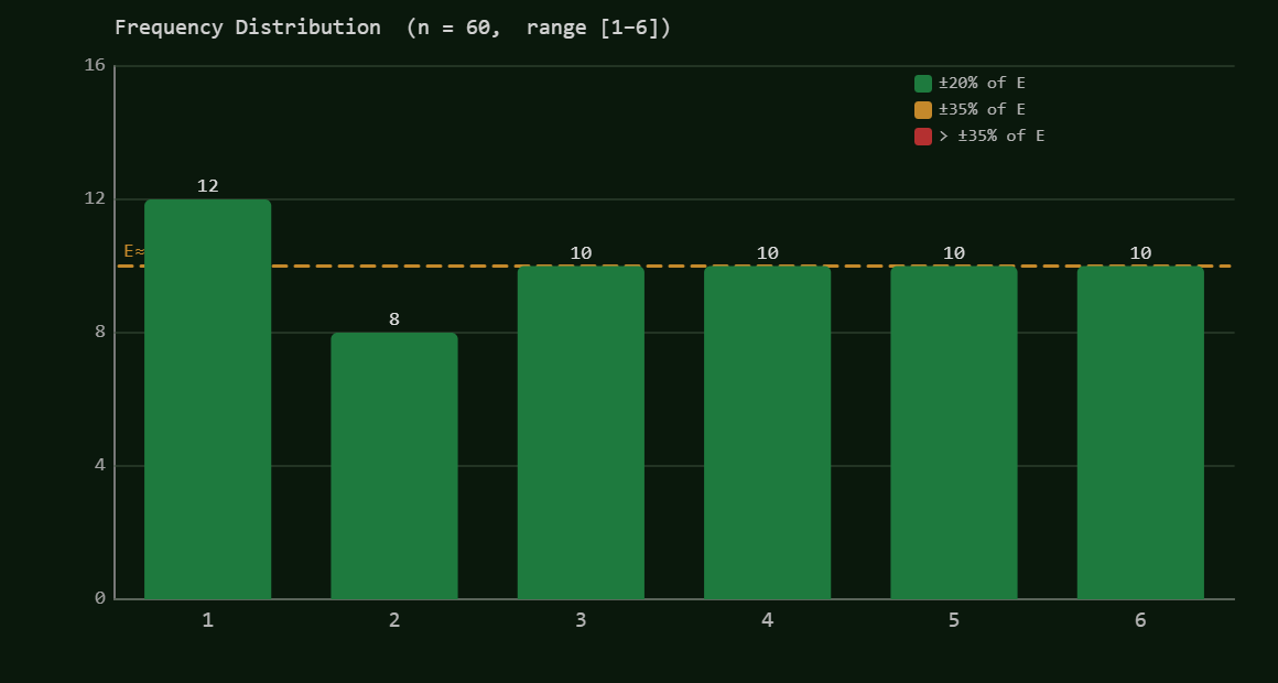
Example 1 — The worked example above: paste this and get X² = 0.80
This 60-value dataset produces the exact counts shown in the table above: value 1 appears 12×, value 2 appears 8×, values 3–6 appear 10× each. Paste into the app with model 1–6; you should see X² ≈ 0.80 and p ≈ 0.98 — no evidence against randomness.
Frequency Histogram — what the Loaded Dice Analyzer shows for this dataset:
images/chi_square_balanced_histogram.png
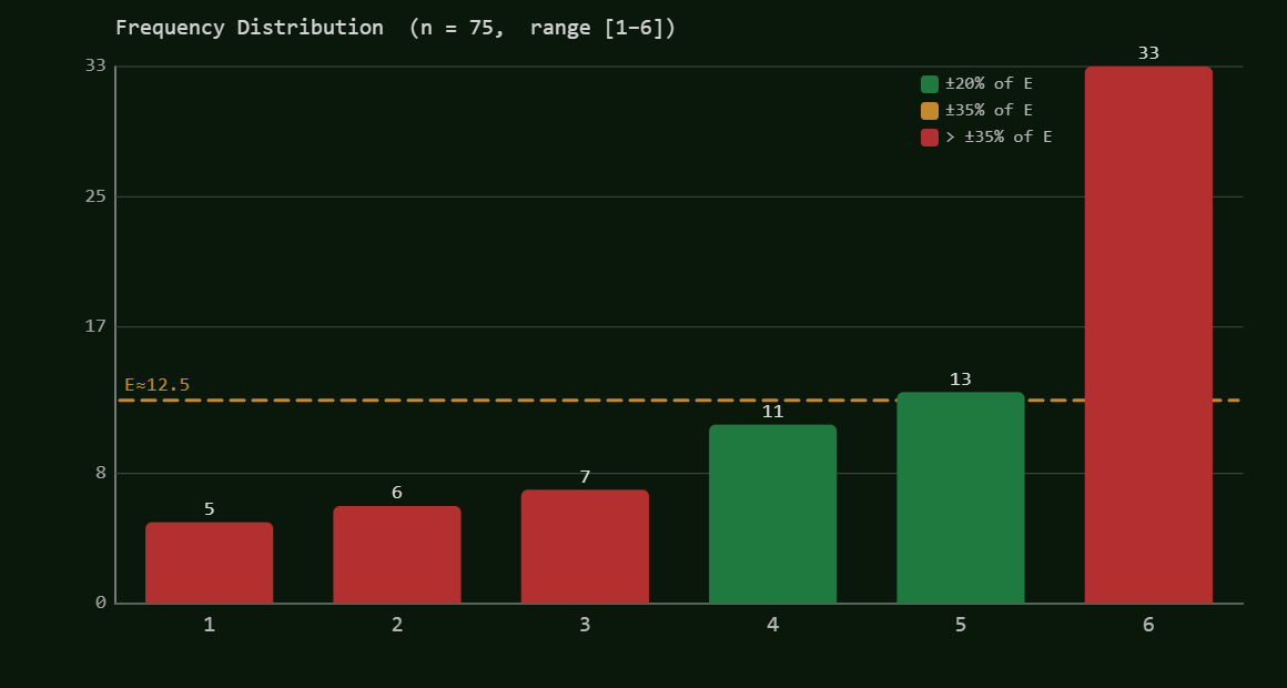
Example 2 — Biased toward 6: value 6 appears far more than expected
Model 1–6, 75 values. Value 6 dominates the distribution. X² ≈ 44, p < 0.000001 — strongly FAILS. Chi-square catches the imbalance immediately.
Frequency Histogram — Example 2: the 6-bar towers above the rest
Example 3 — All fives: the extreme case
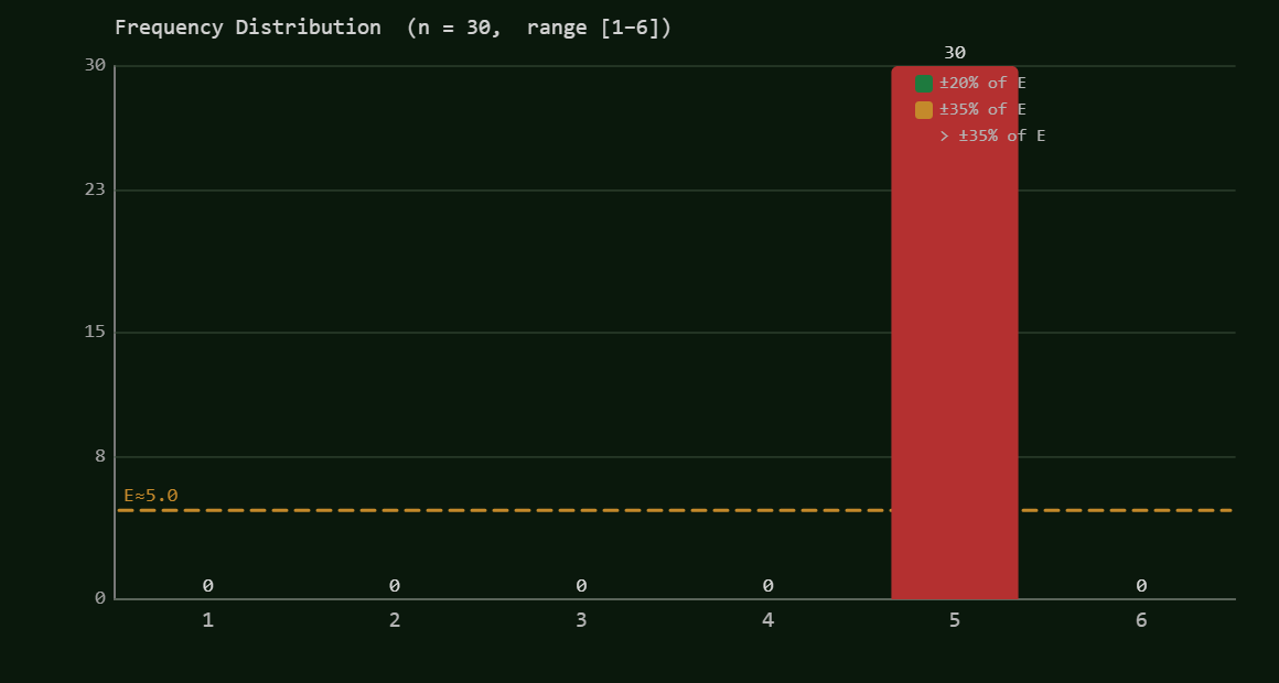
30 identical values. Model 1–6. X² = 150, p ≈ 0. Only one outcome appears; five are absent entirely. Dramatic fail. (Note: X² = 375 for 75 identical fives — chi-square scales with sample size.)
Frequency Histogram — Example 3: one lone tower, five empty bars
Streak Detector
Too much clustering? Too much alternating?
Split each value into two teams: Low (1, 2, 3 ≤ midpoint 3.5) and High (4, 5, 6). Now look for unbroken stretches of the same team — called “runs.” A truly random sequence mixes them up, but not too perfectly. Real randomness has some clumping, some alternating — not extreme either way.
Key Idea
Count the runs R. Compare to what you’d expect under random shuffling. Too few = suspicious clustering. Too many = suspicious alternation. Use a z-score to measure how far R is from its expected value.
Example 1 — All lows, then all highs: extreme clustering
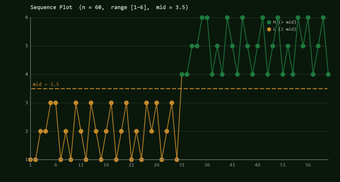
30 Low values followed by 30 High values — exactly 2 runs. Model 1–6. Runs test: R = 2, p ≈ 0. The app will flag this immediately.
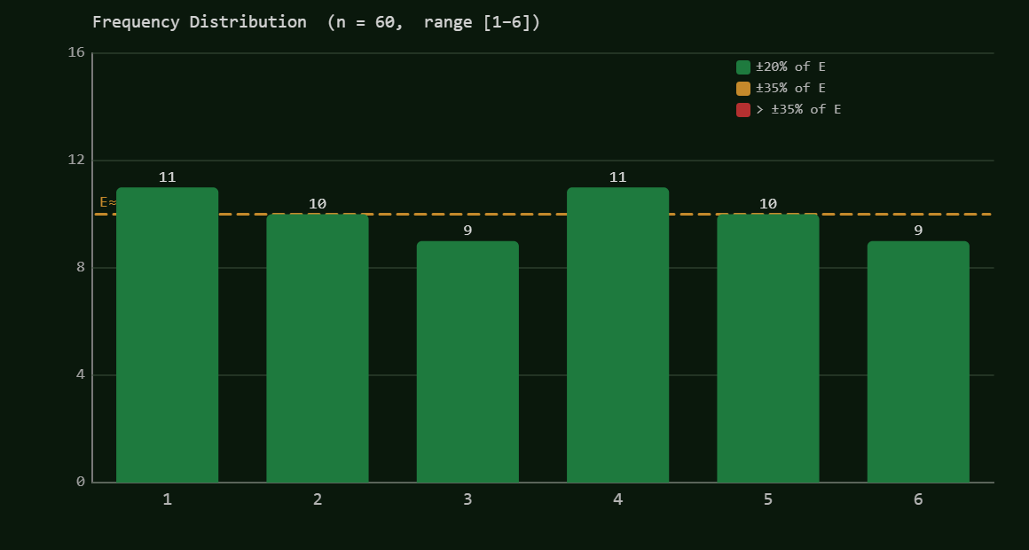
Frequency Histogram — chi-square says: nothing wrong here
Sequence Plot — the runs test says: wait a minute…
The histogram gives this data a clean bill of health. All six bars are green, counts [11, 10, 9, 11, 10, 9] are all within ±20% of expected. Chi-square scores this as completely unremarkable. If frequency were the whole story, you’d never guess anything was wrong.
Now look at the sequence plot. The dashed midpoint line (3.5) divides the dots: amber is Low (≤ 3.5), green is High. See it? The entire left half of the sequence is amber — 30 consecutive Low values. Then the color switches, and the entire right half is green — 30 consecutive High values. That’s just 2 runs where a random sequence would produce about 31. The histogram counted the totals and saw nothing. The sequence plot reveals the block structure in one glance. This is exactly why you need both tests.
Example 2 — Perfect alternation: L,H,L,H every single step
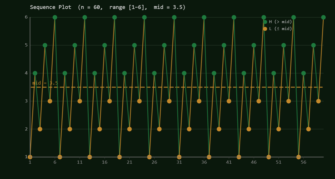
Strict L/H/L/H… pattern — 60 runs (every value is its own run). Model 1–6. Runs test: p ≈ 0, z ≈ large negative. Too perfectly alternating to be random.
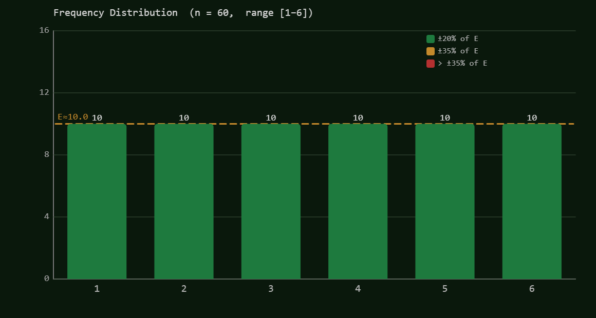
Frequency Histogram — chi-square says: suspiciously perfect
Sequence Plot — the runs test says: nobody alternates like this
Look at the histogram: every single bar lands exactly at 10 — a flawless X² = 0. Not close to expected, not approximately equal — identical. Chi-square is so unbothered it can’t even register a complaint. Ironically, a truly random sequence almost never looks this perfectly balanced; real randomness has natural bumps and dips. But chi-square only knows how to detect too much imbalance — it has no way to flag “too perfect.”
Now look at the sequence plot. Every green dot (High) is immediately followed by an amber dot (Low), and back again, without a single exception — 60 runs in 60 values. Where Example 1 had two massive blocks, this one has sixty tiny blocks, each of length one. A real die doesn’t consciously alternate to avoid repetition; it has no memory. This mechanical back-and-forth is the hallmark of a rule, not randomness. The runs test catches it: R = 60, expected ≈ 31, z ≈ −14. The histogram was blind; the sequence plot makes it obvious in a single glance.
TRICK: Period-10 sequence PASSES the runs test — but isn’t random!
This is the 10-number cycle 1,2,4,5,3,2,6,5,3,4 repeated 6×.
The runs count R ≈ 36, close enough to expected that the test
passes (p ≈ 0.19).
It’s a deterministic repeating cycle — but the runs test is fooled.
A different test (Test 3 at lag 10, or Test 4) will catch it.
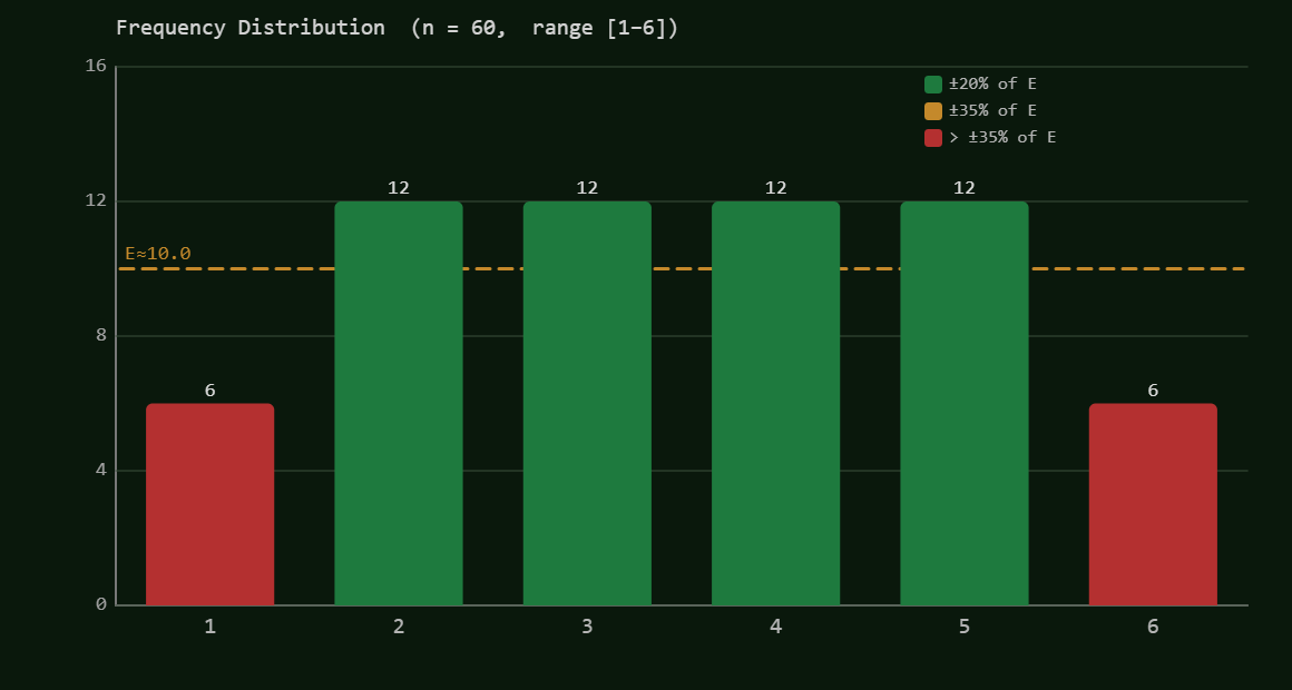
Frequency Histogram — chi-square: a whisper of suspicion, not a shout
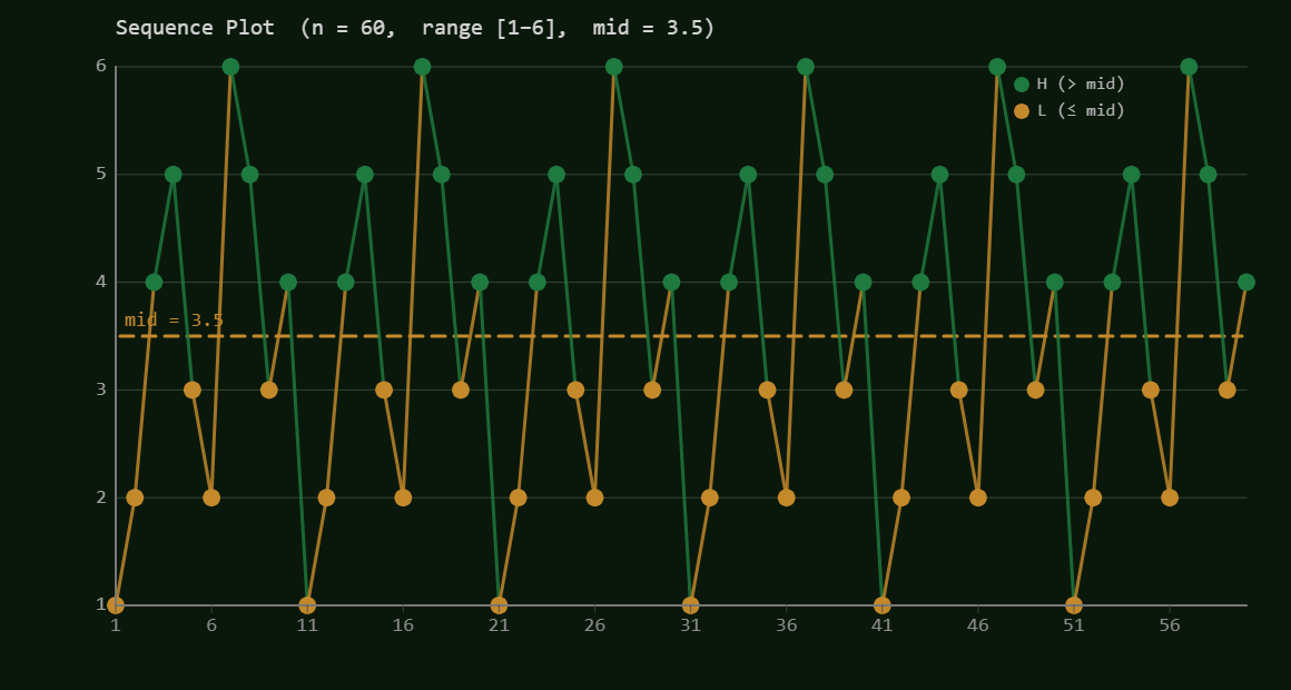
Sequence Plot — runs test: nothing obviously wrong — and that is the problem
Compare this histogram to Examples 1 and 2. The first two had all-green bars — chi-square gave them a clean pass. This one is different: values 1 and 6 show red bars (count = 6, about 40% below expected), while values 2–5 are green. Chi-square notices the imbalance — X² ≈ 4.8 — but with p ≈ 0.44 it shrugs and says “that kind of unevenness happens by chance almost half the time.” A flag without an alarm.
Now compare the sequence plots. Example 1 showed a stark amber block then a green block. Example 2 showed a mechanical green-amber-green-amber zigzag. This one? The green and amber dots appear to mix — no obvious wall, no obvious alternation. The runs count lands near enough to expected that the test nods and moves on. To the eye, and to both tests, this sequence could plausibly be random.
But it isn’t.
It’s the same 10-value cycle —
1, 2, 4, 5, 3, 2, 6, 5, 3, 4
— repeated exactly six times. The sequence has zero randomness; it’s
a clock. Yet chi-square didn’t catch it, and the runs test didn’t catch it.
This is the moment that demands the next two tests. Counting frequencies wasn’t
enough. Counting runs wasn’t enough. To catch a repeating cycle you need to ask
a sharper question: does each value echo itself at a specific distance?
That’s exactly what Test 3 — the Echo Hunter — does.
Echo Hunter
Do values remember where they came from?
In a truly random sequence, knowing roll #1 tells you nothing about roll #2. Or #11. Or #101. Autocorrelation asks: is there a distance at which values echo each other? If value 10 tends to be close to value 20, and value 11 to value 21, something is repeating with period 10.
Key Idea
Pick a lag k. Pair up each value with the one k positions later. Compute the correlation of these pairs. Near +1 → they tend to match. Near −1 → they tend to oppose. Near 0 → no pattern at that distance.
Worked Lag Table — Period-10 Example (n = 60)
For n=60: reference bands are ±1.96/√60 ≈ ±0.253.
| Lag k | rk | Suspicious? (band ≈ ±0.253) |
|---|---|---|
| 1 | 0.076 | No — inside band |
| 5 | −0.200 | Borderline — approaching band edge |
| 10 | 0.833 | YES — strong repetition at exactly lag 10! |
TRICK: Passes lag-1 but FAILS lag-10 — the hidden cycle
Same period-10 data. The lag-1 autocorrelation r1 ≈ 0.076 (well inside reference bands). But r10 ≈ 0.833 — a correlation of 0.83! The sequence is effectively identical to itself when shifted by 10 positions. Lag 1 is completely blind to this. This is why the app checks multiple lags. Use Test 4 (toggle on) to really nail this one.
Example 1 — Consecutive echo: strong lag-1 correlation
Consecutive pairs stay close to each other throughout (5,6, 5,6, … then 4,5, … etc.). The lag-1 autocorrelation r1 will be large and positive — knowing the current value helps predict the next. Model 1–6.
Pair Inspector
What comes after what? (The hardest test to fool)
This test is off by default. Activate it with the Test 4: Ordered-Pair toggle in the Loaded Dice Analyzer before clicking Analyze. When on, it adds a fourth test card and adjusts the score weights.
All the previous tests treat each value somewhat independently: how many times each value appears, how they alternate, how they correlate. But what if the transition from one value to another is biased? What if after rolling a 3, you almost always roll a 5 or 6? The first three tests would never notice — but the Pair Inspector would catch it instantly.
Key Idea
Build a 6×6 grid where cell (i,j) counts how many times value i was immediately followed by value j. Under a fair random model, all 36 cells should be filled roughly equally. The heatmap makes biased transitions visually obvious.
TRICK: Three tests PASS — Pair Inspector FAILS (n = 60)
Same period-10 cycle. Only 5 of 36 possible pairs ever appear. With Test 4 off: chi-square ≈ passes, runs passes, score ≈ 87. Toggle Test 4 on — watch the score drop and the amber FAIL card appear. X² ≈ 186. (App will show E<5 note because n=60 is below 360 threshold.)
Ordered-Pair Heatmap — Test 4 says: five paths, thirty-one dead ends
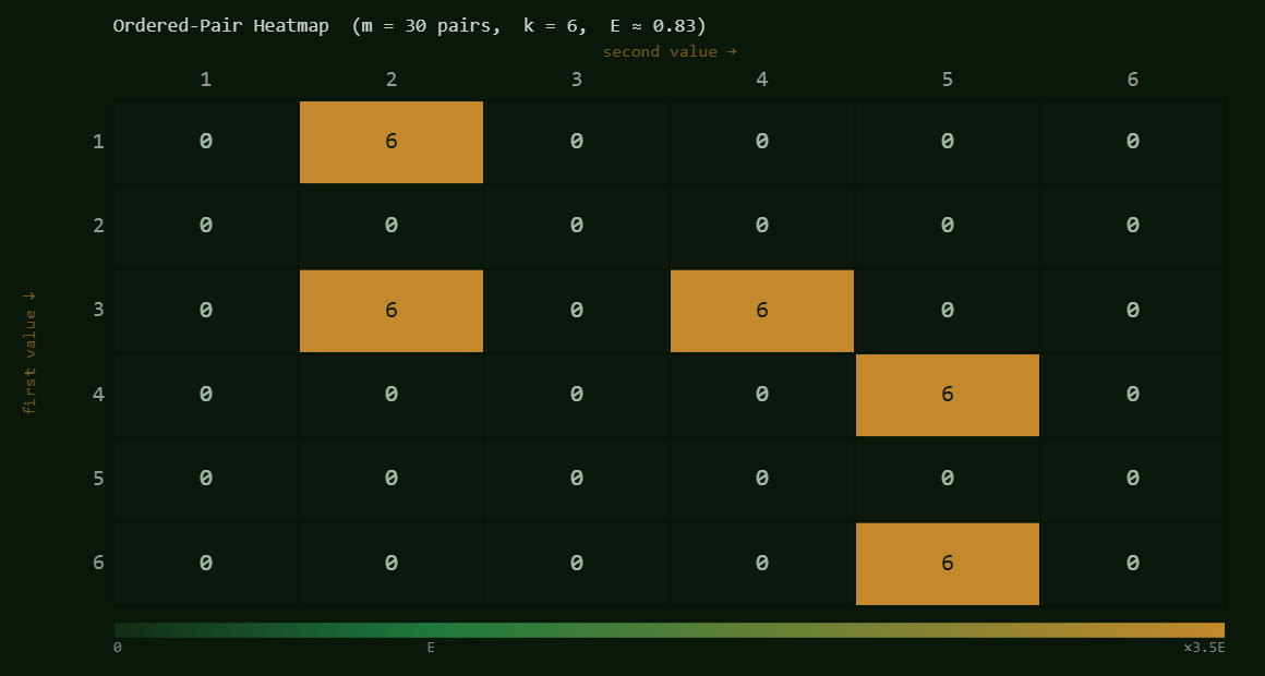
Each row is a “from” value; each column is a “to” value. In a truly random sequence, all 36 cells would glow roughly equally. Here, only 5 of 36 cells are lit — everything else is zero. The map is almost entirely dark. Read it like a transit diagram:
- After a 1, the next value is always 2. No exceptions.
- After a 3, the next value is always 2 or 4.
- After a 4, the next value is always 5.
- After a 6, the next value is always 5.
- Rows 2 and 5 are entirely dark — 2 and 5 never start a pair.
This is the rigid wiring of a 10-value clock. A real die has no memory; it doesn’t “know” what it just rolled. But this sequence does — it always follows the same script. The three other tests handed it a passing grade. Test 4 exposes the script in a single image.
Note: E ≈ 0.83 per cell (n=60, 30 non-overlapping pairs, 36 cells). The E < 5 approximation warning will appear in the app. The chi-square statistic is still informative here because the departure is so extreme — X² ≈ 186 — but for borderline cases, a larger sample is needed for a reliable p-value. The n=600 example below solves this.
Example 1 — Period-10 cycle × 60: clean fail, no approximation warning (n = 600)
The same 10-value pattern repeated 60 times. E = 8.33 per cell — no E<5 warning. X² ≈ 1860, p ≈ 0. Five occupied cells in the heatmap (one per transition pair), each with count = 60. Thirty-one cells are completely empty. Toggle Test 4 ON before analyzing.
Ordered-Pair Heatmap — same five routes, ten times the evidence — and now E ≥ 5
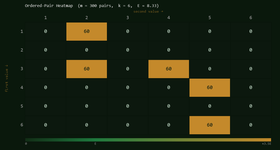
Compare this heatmap to the n=60 version above. The structure is identical — the same five cells are lit, the same 31 are dark. What changed is the evidence: each occupied cell now shows count = 60 instead of 6, and E = 8.33 instead of 0.83. That single change eliminates the E < 5 caveat. The chi-square approximation is now fully valid — no warning, no asterisk. X² ≈ 1860, p ≈ 0.
But here is what makes n=600 the “full collapse” case: the ordered-pair test is no longer the only one raising its hand. With ten times the data, the other tests have enough evidence to speak too:
| Test | n=60 | n=600 |
|---|---|---|
| Chi-square | p ≈ 0.44 — passes | p ≈ 0 — fails (X²=48) |
| Runs | p ≈ 0.19 — passes | p ≈ 0 — fails (z≈17) |
| Autocorrelation | p ≈ 0.56 — passes | p ≈ 0.063 — borderline |
| Ordered-pair | p ≈ 0 — fails * | p ≈ 0 — fails (valid) |
* E < 5 at n=60; approximation unreliable for borderline cases. At n=600, every test tells the same story. Only the autocorrelation lag-1 holds on — barely — because lag-1 still can’t see the period-10 repetition. Score: 22 (F). The detective needed more witnesses. At n=600, it has them.
TRICK: “Never repeat your last value” — empty diagonal
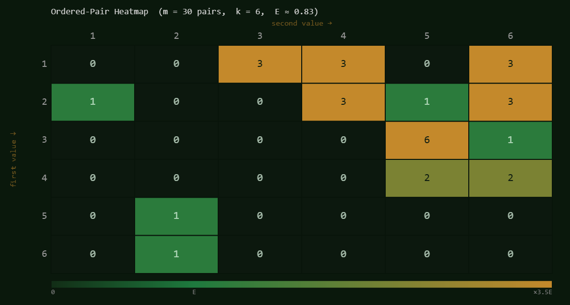
This sequence is constructed so no value is ever immediately followed by itself — a very common human “fairness” bias. Individual frequencies are balanced (chi-square passes), but the runs test fails and the Pairs Heatmap shows a completely dark main diagonal. A true random sequence sometimes repeats — enforcing no-repeats breaks that in ways two of the other tests can detect.
Ordered-Pair Heatmap — Test 4: the main diagonal is entirely dark
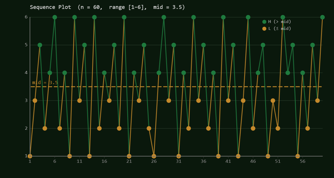
Sequence Plot — Runs test: too many transitions for a fair die
Chi-square: passes. Each value appears roughly 10 times. The frequency histogram would show all-green bars near E = 10. Counting totals reveals nothing wrong.
Heatmap: the empty diagonal. Look at the 6×6 grid — the cells (1→1), (2→2), (3→3), (4→4), (5→5), (6→6) are all zero. Every other cell with any count is off-diagonal. The rule “never follow a value with itself” is written directly into the heatmap. A truly random die sometimes rolls 5 followed by 5; in fact, that should happen about 1 in 6 rolls. Here it never happens.
Runs test: fails — and here is why. Look at the sequence plot. Green and amber dots alternate far more frequently than you’d expect from a fair die. This is not a coincidence: it is a mathematical consequence of the no-repeat rule.
Think about it from a Low value (1, 2, or 3). You cannot stay on the same value, so the next value is chosen from the remaining five. Two of those five are Low; three are High. That gives a 60% chance of switching to High — not 50%. Symmetrically, from a High value (4, 5, or 6), three of the five remaining are Low — again a 60% chance of switching. The no-repeat rule silently tips the odds toward L↔H alternation at every single step.
The result: more runs than a fair die would produce. The runs test sees a sequence that alternates L and H too reliably, flags it as suspicious, and rejects. The pair heatmap then explains why: the diagonal exclusion is what creates the bias. The two tests are telling the same story from different angles.
Example 2 — 600 digits of π: the test has nothing to flag
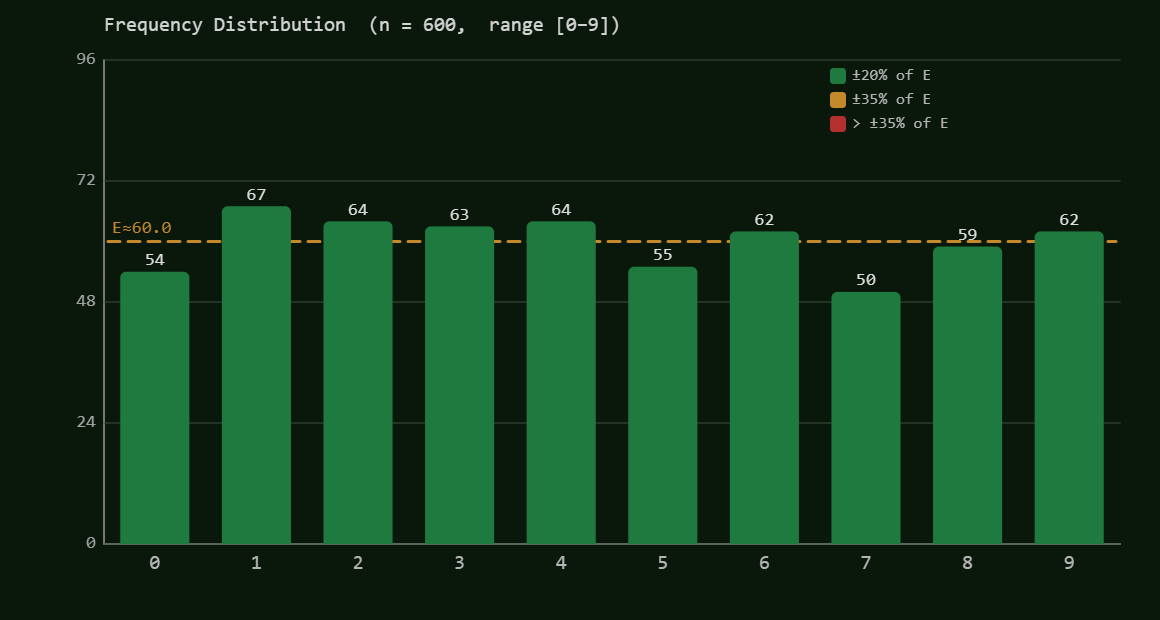
The first 600 decimal digits of π (after the 3.), computed precisely. Model: 0–9 (set Expected Min = 0, Expected Max = 9). Chi-square: X² ≈ 4.33, p ≈ 0.89 — all 10 digit bars are green. Ordered-pair: E = 3.0 per cell (E < 5 note will appear; for a clean test, try 1000 digits). π is completely determined by mathematics — yet all four tests find nothing suspicious. Passing tests does not mean random. It means undetected.
mpmath
• piDigits600.txt
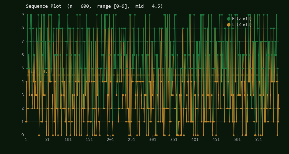
π is conjectured (but not proven) to be a “normal” number — meaning its digits are equidistributed across 0–9 in every block length. For 600 digits, two tests (runs and ACF) flag a slight excess of L↔H alternation. See the images below. Set Expected Min = 0, Expected Max = 9 before analyzing.
Frequency Histogram — chi-square says: beautiful — all ten digits appear roughly equally
Sequence Plot — runs test says: too much alternation for 600 steps
Ordered-Pair Heatmap — pairs test says: no concentrated hot spots — passes
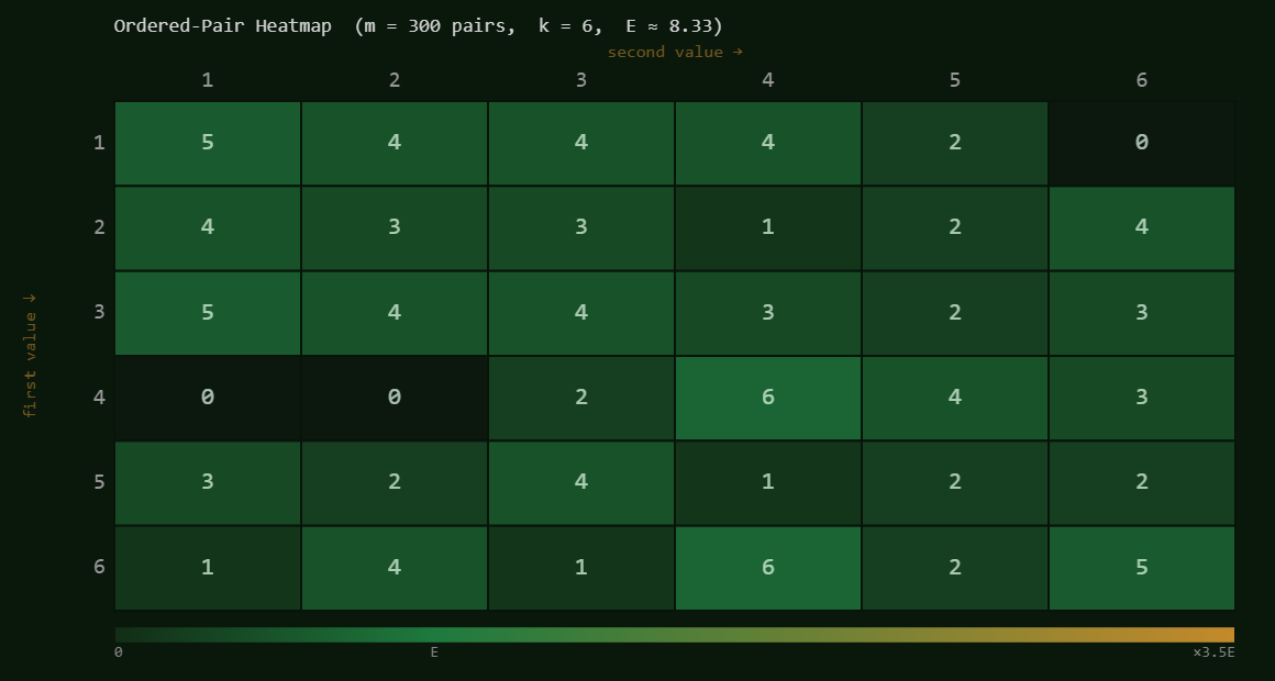
⚠ If your heatmap shows k = 6 instead of k = 10, check that Expected Min = 0 and Expected Max = 9 are set before clicking Analyze & Pairs Heatmap.
The histogram is all green — chi-square passes easily (X² ≈ 4.33, p ≈ 0.89). But the sequence plot shows that pi’s digits alternate L and H more than pure randomness would produce. R = 335 observed runs vs. μ = 300.5 expected (z = +2.82, p ≈ 0.005): runs test fails. ACF lag-1: r⊂1⊂ ≈ −0.104, slightly outside the ±0.080 reference band (p ≈ 0.011): ACF marginal fail. Both tests are detecting the same thing from different angles.
With Test 4 on, the score rises to ≈55 because the ordered-pair test passes — the heatmap is roughly uniform. Adding a passing test raises the average score, even when others fail.
Pi’s normality is a conjecture about the infinite sequence. The first 600 digits are not required to pass every test. This is the lesson: passing tests means “no red flag found,” not “proven random.” And failing them means “evidence found,” not “proven non-random.”
Case Study: The Look-and-Say Mystery
A student submitted 73 values claiming they came from a random 3-outcome model (values 1, 2, 3). Let’s run the app and see what it finds.
| Test | Result |
|---|---|
| Chi-square | X² = 24.85, p = 0.000004 — REJECTED |
| Runs (1 vs {2,3}) | R = 39, p ≈ 0.54 — passes |
| Autocorrelation | Largest at lag 2: r2 ≈ −0.287 — notable |
| Pattern detected? | Yes — but which pattern? |
Paste the data below into the app with model min = 1, max = 3:
The source was the Look-and-Say sequence! Each term describes the digit groups in the previous term: 1 → 11 → 21 → 1211 → 111221 → 312211… Reading the digit stream (1,1,1,1,2,1,2,1,1,… and so on) produces far more 1s than 2s or 3s, because “one of something” is the most common description.
Lesson: The chi-square caught the frequency imbalance without knowing anything about Look-and-Say sequences. A statistical test can detect that something is wrong without knowing why. That’s its power — and its limitation.
Case Study 2: The Square Root of 2
π tested us — it scored ~45 and surprised everyone. Let’s try √2. Irrational like π, conjectured normal like π, but computed a completely different way. Will it behave better?
√2 = 1.41421356237… — its decimal digits never repeat and never end. We computed 1000 digits using Newton’s Method (the same derivative-based iteration from AP Calculus) and applied all four tests with model 0–9. With n=1000 and k=10, the ordered-pair test gets E = 5.00 per cell — exactly at the threshold, no approximation warning. How we computed the digits →
1000 digits of √2 — all four tests pass cleanly
Model 0–9. Set Expected Min = 0, Expected Max = 9. Toggle Test 4 ON before analyzing. Expected results: chi-square X² ≈ 8.38 (p ≈ 0.50), runs z ≈ −0.38 (p ≈ 0.71), ACF r⊂1⊂ ≈ 0.030 (p ≈ 0.34). Score ≈ 100.
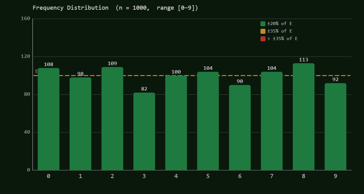
Frequency Histogram — all ten bars green: natural variation, nothing alarming
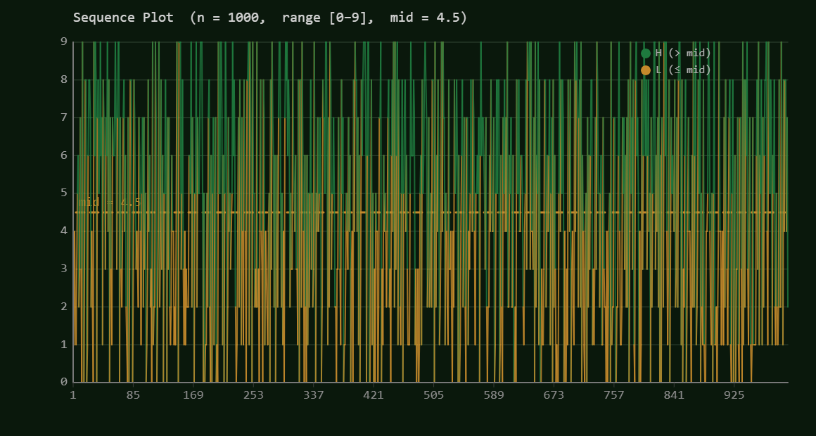
Sequence Plot — 1000 points, genuinely mixed: no blocks, no alternation, no pattern
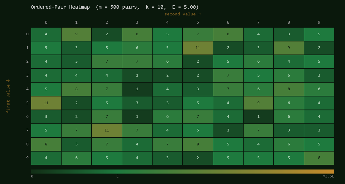
Ordered-Pair Heatmap — all 100 cells occupied, roughly uniform warmth: this is what random looks like
Histogram (top): all ten bars are green, counts 82–113 vs. expected 100. The digit 3 bar (82) is the lowest, but 82/100 = 0.82 — just inside the ±20% zone. Natural sampling variation, nothing more. Chi-square X² = 8.38 confirms it.
Sequence plot (middle): 1000 dots at this scale compress heavily — each dot is tiny. What you want to see is a uniform salt-and-pepper mix of amber and green across the full width, with no obvious blocks (like Example 1 in the Streak Detector) and no obvious alternation (like Example 2). That’s exactly what you see here. The runs test passes (z = −0.38, p ≈ 0.71): 495 observed runs vs. 501 expected.
Heatmap (bottom): m = 500 pairs, k = 10, E = 5.00 — the first heatmap in this tutorial with no E < 5 caveat. Look at every cell: every one of the 100 possible digit-to-digit transitions appears at least once. Most counts are 1–9, three cells reach 11 (ratio 2.2 × E — well within the green color zone). There are no dominant transitions, no empty rows or columns, no structure at all. This is what the heatmap looks like when the digits have no memory of each other.
Compare this heatmap to the period-10 sequence heatmap: 5 bright gold cells and 31 dark empty cells. The visual contrast between those two images is the clearest possible demonstration of what Test 4 catches and what it looks like when there’s nothing to catch.
| Test | π (600 digits) | √2 (1000 digits) |
|---|---|---|
| Chi-square | p≈0.89 — passes | p≈0.50 — passes |
| Runs test | p≈0.005 — fails | p≈0.71 — passes |
| Autocorrelation | p≈0.011 — fails | p≈0.34 — passes |
| Score (3-test) | ≈45 (C) | 100 (A) |
Neither result is surprising to a statistician. Both numbers are conjectured to be normal — but “conjectured normal” is a statement about the infinite sequence, not a guarantee for any particular finite sample. π’s first 600 digits happen to alternate L and H more vigorously than expected. √2’s first 1000 digits happen to look quite clean. A different window on either number might tell a different story. This is why “passes tests” means “no evidence found”, not “proven random.”
The Big Picture: Why Four Tests?
| Test | Question Asked | Blind Spot |
|---|---|---|
| 1. Chi-square | Right frequencies? | Ignores order entirely |
| 2. Runs | Right amount of mixing? | Ignores exact positions and run lengths |
| 3. Autocorrelation | Right distances (linear)? | Linear only; finite lags; misses nonlinear patterns |
| 4. Ordered-pair | Right transitions? | Pairs only — longer blocks require higher-order tests |
No collection of passes proves a sequence is random. Each test finds a specific kind of evidence against randomness. Pass all four and you can say: “No red flags found — yet.” That’s not certainty. It’s just a careful absence of evidence. True randomness is a statement about a generating process, not about the numbers themselves.
Real applications use carefully engineered PRNGs. The simplest is the Linear Congruential Generator (LCG), which uses the rule xn+1 = (a · xn + c) mod m. With good constants, an LCG passes many tests — but it has detectable structure (famous example: consecutive triples from any LCG lie on a finite set of hyperplanes). You can generate LCG data in the Loaded Dice Analyzer’s Sample Generator tab.
The Mersenne Twister (period 219937−1) passes all standard test batteries and is the default in Python, R, and many gaming engines. But it is not cryptographically secure — its internal state can be reconstructed from 624 consecutive outputs.
Cryptographic PRNGs (like ChaCha20 or
window.crypto.getRandomValues()) are designed to resist even
adversarial analysis. For these, our four tests find nothing —
and that’s exactly the point.
See also: the
Butterfly Effect app
for a chaotic PRNG based on the logistic map f(x) = 4x(1−x).