Who Is This For?
You have probably heard people mention the “bell curve” — when a teacher grades on a curve, when a doctor says your height is “in the normal range,” when a news article talks about the distribution of incomes. The bell curve is everywhere.
But why does it show up everywhere? That question has a beautiful answer, and you already have enough math to understand it. If you know how to multiply out (x + y)², you have everything you need.
One Peg — One Coin Flip
Let’s start with the simplest possible version. One peg. A ball drops straight toward it.
The ball hits the peg and bounces left or right. There is nothing special pulling it one way or the other, so each direction happens half the time:
This is exactly a coin flip. Heads vs. tails. Yes vs. no. Left vs. right. One peg gives us two outcomes, each equally likely. Not very exciting yet — but this one idea is the seed that grows into the entire bell curve.
Two Rows — Counting Every Path
Now add a second row. The ball makes two decisions. At each peg it goes Left (L) or Right (R). Since there are two decisions and each has two choices, there are exactly 2×2 = 4 possible paths:
The path counts — 1, 2, 1 — tell us how many ways a ball can reach each bin. Since all 4 paths are equally likely, the probabilities are:
| Bin | Paths | Probability | Percent |
|---|---|---|---|
| 0 (far left) | 1 | 1⁄4 | 25% |
| 1 (middle) | 2 | 2⁄4 | 50% |
| 2 (far right) | 1 | 1⁄4 | 25% |
The middle is already twice as likely as either edge — because there are two different paths that lead there (LR and RL), while the edges can only be reached one way each. This is the seed of the bell shape.
Pascal’s Triangle — The Pattern You Were Looking For
Let’s count paths for 3 rows and 4 rows too. Rather than listing every path, we can notice a shortcut:
The number of paths to bin k in row n equals the number of paths to bin k−1 plus the number of paths to bin k in the previous row.
In plain English: “you either arrived from the left or from the right, so add the counts from both sources.”
That rule builds a famous triangle. Each number is the sum of the two numbers directly above it:
Notice something else: each row adds up to a power of 2. Row 4 adds up to 1+4+6+4+1 = 16 = 24. That makes sense — there are 24 = 16 total paths through 4 rows, and Pascal’s Triangle tells us exactly how they split between the bins.
Your FOIL Skills Pay Off — The Binomial Expansion
Here’s where your Algebra 2 skills connect directly to the board. Let’s label a left bounce L and a right bounce R. A ball going through n rows makes n choices, each L or R.
Now expand (L + R) raised to the power n:
Do those coefficient rows look familiar? They should — they are Pascal’s Triangle.
Here’s what each term means in plain English: the term 6 L²R² in the (L+R)4 expansion means “there are 6 ways to arrange exactly 2 left-bounces and 2 right-bounces in a sequence of 4 total bounces.” Those 6 arrangements are the 6 paths that all land in bin 2 (the middle bin) after 4 rows.
The Formula — Predicting Every Bar Height
We can now write a formula for the probability of landing in any bin. Let’s call the total number of peg rows n, and the bin number k (counting from 0 on the left).
- The total number of paths through n rows = 2n
- The number of paths to bin k = the kth entry in row n of Pascal’s Triangle = C(n, k)
The symbol C(n, k) is read “n choose k” and equals:
Don’t be scared by the exclamation marks — they just mean “factorial.” For example, 4! = 4×3×2×1 = 24. Let’s verify the formula for 4 rows:
| Bin k | C(4, k) | (½)4 = 1⁄16 | P(bin k) | % |
|---|---|---|---|---|
| 0 | 1 | 1⁄16 | 1⁄16 | 6.25% |
| 1 | 4 | 4⁄16 | 1⁄4 | 25% |
| 2 (middle) | 6 | 6⁄16 | 3⁄8 | 37.5% |
| 3 | 4 | 4⁄16 | 1⁄4 | 25% |
| 4 | 1 | 1⁄16 | 1⁄16 | 6.25% |
This is called the Binomial Probability Mass Function (PMF for short). The gold curve in the Galton Board simulator plots exactly this formula for the current number of peg rows — calculated from the formula alone, before any ball has dropped.
The Formula’s Famous Cousin — The Bell Curve Equation
The binomial PMF gives exact probabilities for specific whole-number bins. But mathematicians in the 1700s asked a deeper question: what if the number of rows grew to infinity? What smooth curve would the staircase histogram converge toward?
The answer is one of the most celebrated equations in all of mathematics — the Normal Distribution, also called the Gaussian curve:
Four constants you need to know:
- μ (mu) — the mean; the center of the curve. For our board: μ = n⁄2.
- σ (sigma) — the standard deviation; how wide the curve spreads. For our board: σ = √(n × 0.25).
- π — 3.14159… Yes, the same π from circles and geometry. It appears here because the normal curve, when integrated over all x, must equal exactly 1 — and that calculation involves π in a deep way.
- e — 2.71828… Euler’s number. Like π, it is irrational and arises naturally throughout mathematics. It is the base of natural logarithms and shows up whenever something grows or decays continuously — compound interest, radioactive decay, population growth.
The Secret Lives in the Exponent
The entire personality of the bell curve lives in that exponent, −½z². The variable z is the z-score — the fraction (x−μ)⁄σ — which answers the question: “how many standard deviations away from the center is x?” You will meet the z-score again throughout statistics; it is one of the most useful ideas in the whole subject.
Because z is squared, the exponent −½z² is always zero or negative. Because e raised to a large negative number is tiny, points far from the center have nearly zero height. The table makes this vivid:
| Distance from center | z-score | Exponent −½z² | e−½z² | Relative height |
|---|---|---|---|---|
| At center (μ) | 0 | 0 | 1.000 | 100% — peak |
| 1σ away | 1 | −0.5 | 0.607 | 61% |
| 2σ away | 2 | −2 | 0.135 | 14% |
| 3σ away | 3 | −4.5 | 0.011 | 1% — nearly zero |
More Rows = Better Bell
With 4 rows the probabilities are: 6.25%, 25%, 37.5%, 25%, 6.25% — a tent shape on paper, but an important limitation applies when we run the physical simulation.
The lesson: the math is exactly right, but a physical device needs enough peg rows to guarantee every ball makes every required decision. This is why real Galton boards have many rows of closely-spaced pegs, and why the simulator’s default is 14 rows.
Let’s skip ahead to 8 rows and see the bell shape becoming clear:
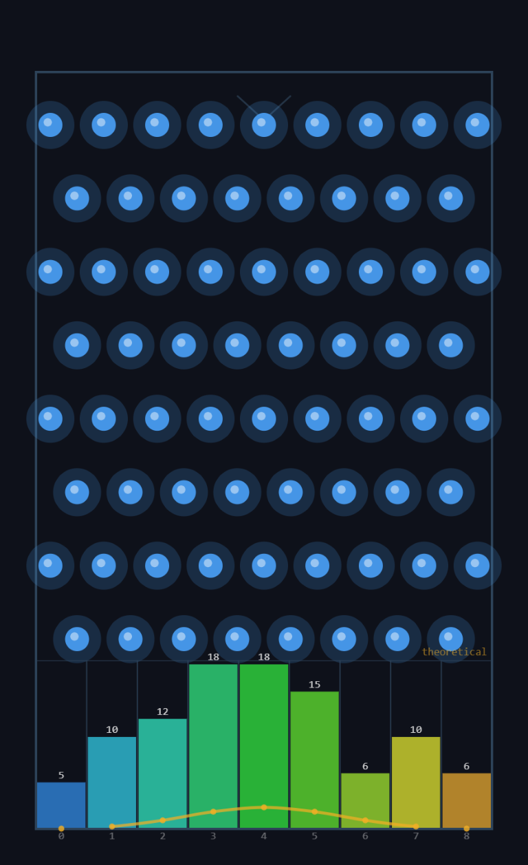
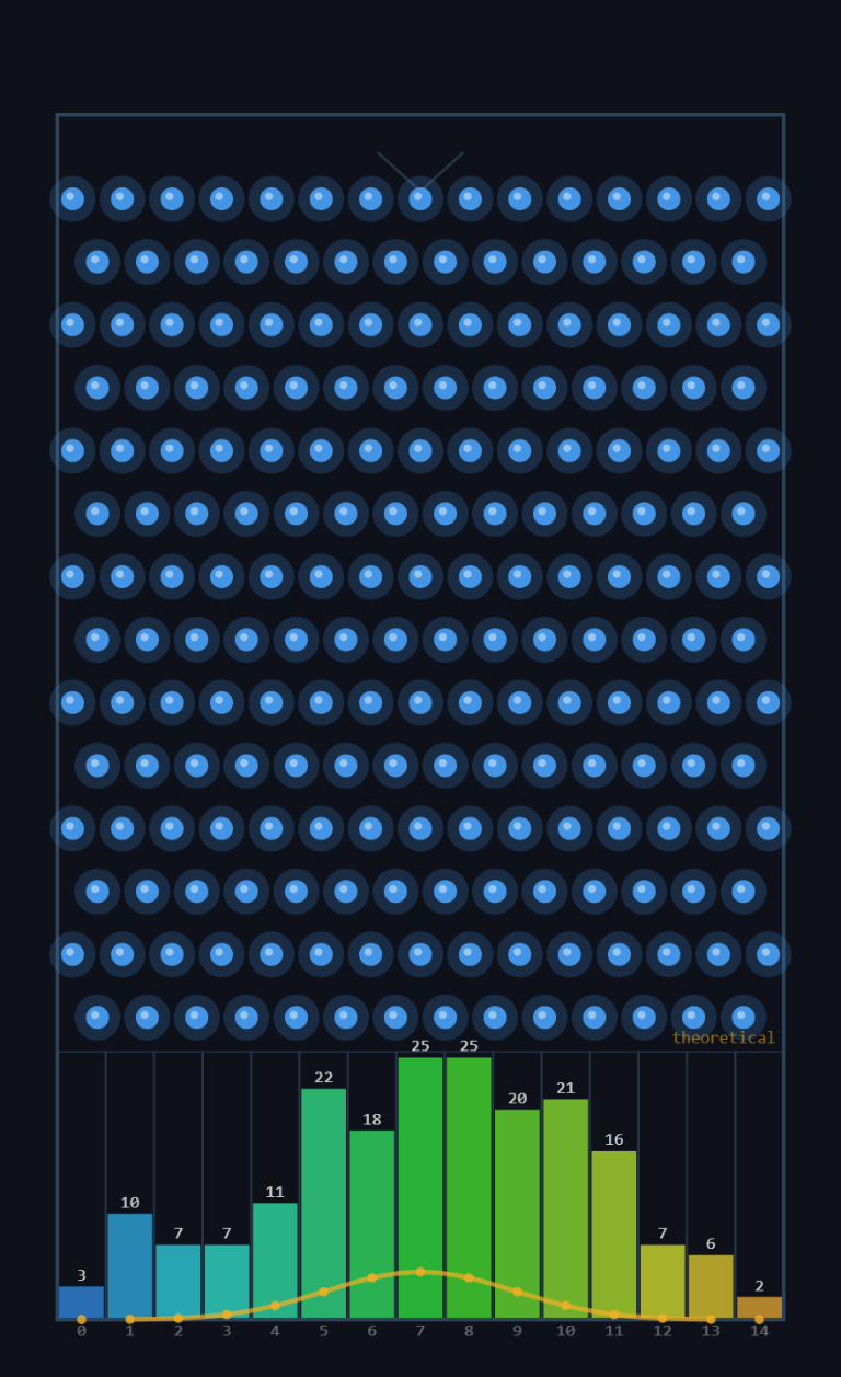
Now watch what happens as we continue to increase the rows. Each additional row adds another binary decision for every ball, pushing the distribution ever closer to the ideal bell curve:
With 14 rows the shape is already the famous bell curve you see in statistics textbooks. Run the simulator with 14 rows and drop 200 balls to see this live:
Why the Middle Always Wins
Here’s the intuition in plain language. To land in the rightmost bin, a ball must go right at every single peg. There is only one path that does that: RRRR…R. There’s only one way to be perfectly consistent.
To land in the middle bin (half lefts, half rights), a ball has many more options. With 4 rows: LLRR, LRLR, LRRL, RLLR, RLRL, RRLL — that’s 6 different paths, all ending in the same middle bin.
The middle bin wins because there are more ways to be average than to be extreme. This is not just a math fact — it’s a truth about the world. There are many more ways to be of average height than to be seven feet tall. Many more ways to score near the class average than to get a perfect score. The bell curve is nature’s way of showing that balance is always more common than extremes.
Data Chases the Formula
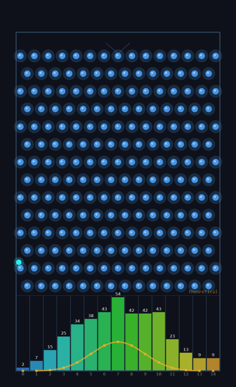
Here is one of the most satisfying things you can watch in all of statistics. Drop 200 balls. The empirical histogram (the actual bars) already looks close to the gold curve. Drop 200 more. Closer. Drop 200 more. Even closer.
The random data converges toward the mathematically predicted shape. It never reaches it perfectly — randomness always leaves some wiggle room — but it keeps getting closer as the sample size grows.
In the statistics panel, watch the Mean Bin and Std Dev rows converge toward Predicted Mean and Predicted σ as balls accumulate. Those predicted values come purely from the formula — they were calculated before a single ball dropped.
The Big Idea — Why This Matters Beyond Pegs
The Galton Board works because every ball makes a sequence of independent, identical random decisions. What happens when you apply the same logic outside of a machine?
- Heights of people: Your height is the sum of many small genetic effects, each acting somewhat independently. Add up many small random things → bell curve.
- Test scores: Your score is the sum of whether you happened to know each individual question. Many independent yes/no events → bell curve.
- Measurement error in science: The error in any measurement is the accumulation of many small, independent sources of imprecision. Sum of many small errors → bell curve.
- Stock prices, weather patterns, IQ scores, crop yields… wherever you find the sum (or average) of many independent random pieces, you find the bell curve.
Mathematicians proved in the 1800s that this is always true: whenever you add up enough independent random things, the result always approaches the same bell-shaped curve, regardless of what the individual things look like. This result is called the Central Limit Theorem — arguably the most important single idea in all of statistics.
The Galton Board is the world’s most beautiful visual proof of this theorem. Every ball drop is a mini-experiment. Every bin is a vote. After enough votes, the bell wins every time.
Try the Simulator — See It for Yourself
Everything on this page is visible live in the TNT Galton Board Simulator. Some things to try:
Set Peg Rows to 4. Drop 50 balls. Notice the rough tent. Then set Peg Rows to 14 and drop 200 balls. Watch the tent become a bell. The gold curve tells you what to expect before you drop anything.
After dropping 200 balls, compare Mean Bin to Predicted Mean and Std Dev to Predicted σ. How close did the data get to the formula? Drop 200 more and check again.
Turn on Ball–Ball Physics. Now balls interact with each other — they are no longer independent. Watch the distribution change. This is exactly why the independence assumption matters.
Reset and switch between Triangle and Rectangle modes. The Triangle mode shows Galton’s original design — notice how the edge bins are taller than the formula predicts. Why? Because some balls escape through the gaps. That’s the edge-effect, and it’s a lesson in model assumptions.
Want to Go Deeper?
The S.P.A.R.K. Chat Log documents the entire development of this simulator — 21+ sessions of design decisions, physics discussions, statistical analysis, and even some debugging adventures. It’s a window into how real programming projects evolve iteratively.