Building the Galton Board Simulator
From a student’s RGB sketch to an HSB-palette, portrait-canvas, statistics-teaching app.
This log documents the build of the Galton Board Simulator — a p5.js interactive that lets students drop balls through a triangular peg array and watch the binomial distribution converge to a bell curve. The project grew from a student-origin sketch (Stranger Things theme, RGB colors) into a TNT-standard app with HSBA colors, a portrait canvas, and a full statistics control panel.
Designed as a dual-audience tool: CS students see p5.js physics, HSBA color design, and the module pattern; AP Stats students see the Central Limit Theorem emerge in real time.
You are a web developer, high school computer science teacher and AP Stats teacher and a co-creator here at TNT. You have looked at a former app done by a student (loading icons) and are very familiar with our SPARK process where we document our app developments and use them with our novices to teach them how to ‘vibe code.’ I’ve attached our SPARK method docs and CRAFT prompting techniques. We’d like to use David’s app as a basis for a new app, galtonBoardSimApp.html with associated files galtonBoardSimAppStyles.css, galtonBoardSimAppSketch.js, and galtonBoardSimAppScripts.js. We’ve got a parent folder and a suggested sketch, galtonBoardOrigSketch.js that can be used as a starting place for our p5js sketch associated with this app. This HTML/CSS/Bootstrap5/JavaScript p5js app should serve as a training ground for computer science students learning JavaScript and Processing p5js and an inspiration for AP Stat students learning about ‘the bell curve.’ I’ve got a hero image for the hero background you can use for a color palette. Unlike the original script, we want to use HSBA not rgb in our design. This will be our first prompt in the series, and as we did in other chatlogs (I attached two) I want to include my prompts and your grade/critique of them along with the work you do to get our final working app. The canvas should be on the right and the controls should be on the left. I’d like to be able to influence the pertinent parameters of the simulation including speed, gravity, number of pegs, peg spacing, etc. The canvas can be oriented as portrait to accommodate the pegs and the collection bins in the bottom of the canvas. Let’s get an initial version up and running and we can tweak it from there.
We’ll want galtonBoardSimAppChatlog.html along with its style sheet.
C — Context: Excellent. Six tagged files deliver the full workspace: the original student sketch (physics logic to adapt), David’s app (page structure template), two chatlogs (SPARK format reference), and two SPARK/CRAFT documentation pages. The hero image as palette source is an efficient way to establish visual identity without enumerating color codes — it delegates the palette extraction to the AI while anchoring the design intent in a concrete image.
R — Role: Three named, all relevant. Web developer (implementation), CS teacher (novice-accessible code structure), AP Stats teacher (bell curve pedagogy). Naming all three simultaneously signals that every design decision should serve all three lenses. The “co-creator at TNT” addition establishes shared ownership of the aesthetic conventions.
A — Action: Multi-layered and correctly sequenced. Build six files. Use David’s app as template. Start from the existing sketch. Expose specific simulation parameters. Document as SPARK Session 1. The phrase “let’s get an initial version up and running and we can tweak it from there” correctly sets expectations: this is a first-pass build, not a finished product. That framing prevents over-engineering in Session 1.
F — Form: Explicit and cross-referenced. All six file names given. Layout specified (controls left, canvas right — the opposite of David’s app). Portrait canvas explicitly motivated (needs height for pegs + bins). SPARK format by reference to the two attached chatlogs, which is more efficient than re-describing the format.
T — Tight Constraints: One critical, one implied. “HSBA not RGB” is the critical constraint — it determines how every color is specified in the sketch. “Portrait orientation” is the implied constraint, with a clear physical rationale (pegs cascade vertically into bins at the bottom). Minor gap: the list of parameters (“speed, gravity, number of pegs, peg spacing, etc.”) leaves the “etc.” open — a slightly tighter list would avoid guessing. Addressed in the R section.
The hero image (robotGaltonBoard1.jpg) shows a STAT-BOT robot presenting a Galton Board to enthusiastic students in a statistics classroom. The dominant colors extracted and converted to HSB:
--gb-bg:     HSB(222, 45, 10)   →  near-black navy   (classroom shadows)
--gb-blue:   HSB(210, 75, 80)   →  steel blue        (STAT-BOT body color)
--gb-gold:   HSB(40,  85, 95)   →  warm amber/gold   (classroom lighting, ball colors)
--gb-light:  HSB(210, 15, 95)   →  near-white        (whiteboard, clean text)
--gb-card:   HSB(222, 40, 16)   →  dark blue-gray    (control card backgrounds)
Ball colors use HSBA with 8 hues spread evenly across the wheel (0, 45, 90, 135, 180, 225, 270, 315), all at S=85, B=95. This produces a rainbow that maps naturally to the bins across the board — the bell curve emerges as a color gradient from the edges toward the center.
The original student sketch used RGB arrays for every color: [233, 69, 96] for pegs, [255, 0, 128] for ball colors. These numbers are opaque — you cannot tell by reading them whether the color is warm or cool, vivid or muted.
With colorMode(HSB, 360, 100, 100, 100):
HSB(210, 75, 80)  →  "a moderately saturated steel blue at 80% brightness"
HSB(40,  85, 95)  →  "a vivid warm amber at near-maximum brightness"
HSB(0,   85, 95, 60) →  "a vivid red at 60% opacity"
This is readable, designable, and directly connected to the color theory students learn when they study UI design. Ball hues can be spread evenly across the wheel with hue = i * (360 / numBallColors) — a formula that is immediately understandable in HSB and completely opaque in RGB.
The Galton Board is physically tall: pegs cascade down row by row, and the collection bins need headroom to show growing histograms. A landscape canvas forces the peg spacing to be compressed horizontally, making the cascading physics hard to see. Portrait gives:
- Enough vertical travel for physics to feel realistic (balls noticeably accelerate)
- Room for up to 16 peg rows without crowding
- Collection bins with bars tall enough to display meaningful height differences
- A natural top-to-bottom reading direction that mirrors how a real Galton Board works
At 440×720, the canvas fits in the right column of a Bootstrap row on tablet and desktop, with controls in the left column. On mobile it stacks naturally.
The prompt listed “speed, gravity, number of pegs, peg spacing, etc.” The “etc.” was resolved by asking: what would an AP Stats teacher and a CS student each want to control?
| Parameter | Range | Why it matters |
|---|---|---|
| Speed | 0.2–3.0× | Slow down to see individual bounces; speed up to accumulate statistics faster |
| Gravity | 0.1–1.0 | Low gravity: slower fall, more visible bouncing; high: fast dramatic drop |
| Bounce Factor | 0.2–0.9 | Energy retained after peg collision; affects randomness of deflection |
| Peg Rows | 4–16 | More rows = more coin flips = tighter bell curve (CLT in action) |
| Peg Radius | 4–14 px | Visual clarity; larger pegs make collisions more visible |
| Ball Radius | 3–10 px | Ball-to-peg size ratio affects deflection realism |
| Drop Interval | 50–500 ms | Controls crowding; slow interval shows individual trajectories |
galtonBoardSimApp.html — Standard TNT page. Processing active in navbar. Hero with robotGaltonBoard1.jpg overlay. About section explaining Galton, the binomial→normal connection, and the coin-flip model. Two-column layout: controls left (col-lg-4), portrait canvas right (col-lg-8).
styles/galtonBoardSimAppStyles.css — Navy dark background, steel blue accents, warm gold highlights. --gb-* custom properties. Slider groups, control sections, button variants, statistics panel, responsive stack at mobile.
sketches/galtonBoardSimAppSketch.js — Adapted from galtonBoardOrigSketch.js. colorMode(HSB, 360, 100, 100, 100) at setup. 440×720 portrait canvas. All colors as HSBA arrays. Added: bell-curve overlay (golden line showing theoretical binomial PMF), improved bin visualization (stacked ball representation), peg glow effect in HSB. Public API: gbDropBall(), gbDropMany(n), gbToggleContinuous(), gbReset(), gbSet*(v) functions.
scripts/galtonBoardSimAppScripts.js — Slider and button handlers. DOMContentLoaded wiring. 500 ms interval polling to update statistics display from sketch state.
galtonBoardSimAppChatlog.html — This file. SPARK Session 1 with CRAFT critique, design decisions, file inventory.
styles/galtonBoardSimAppChatlogStyles.css — Navy/steel-blue chatlog palette. SPARK banner variants, chat bubbles, annotation boxes, code snaps.
Sir Francis Galton built the first Quincunx board in 1889 to demonstrate that the binomial distribution converges to the normal as n grows. Each ball faces n binary choices (left or right at each peg), each with probability 1/2. After n rows, the ball lands in bin k with probability:
P(bin k | n rows) = C(n, k) × (1/2)^n
This is the binomial PMF with p=0.5. For large n, it converges to N(μ=n/2, σ²=n/4). With 12 peg rows, the distribution is nearly indistinguishable from normal to the eye. With 16 rows and 500 balls, the bell curve emerges unmistakably.
For AP Statistics students: this is the CLT in physical form. The simulation makes the theorem tangible before the abstract proof. For CS students: it shows how randomness in a single simple rule (50/50 at each peg) produces organized structure in the aggregate — the same principle behind many natural phenomena.
RGB is the computer’s color model — it maps directly to hardware (red, green, blue phosphors). HSB is the designer’s color model — it maps to how humans describe color (hue, saturation, brightness). When teaching color in a CS class:
- “Change the hue from 0 to 120” = “shift from red to green” — immediately visible and intuitive
- “Change the saturation from 100 to 20” = “wash out the color” — describable in English
- “Hue = binIndex × (360 / numBins)” = rainbow spread across the histogram — one formula
The original student sketch had 6 hardcoded RGB arrays for ball colors. The HSBA version replaces them with one formula. This is the kind of simplification that makes code both more readable and more maintainable — a real-world CS lesson hiding inside a stats simulation.
The Galton Board is built from a single rule: at each peg, a ball goes left or right with equal probability. This is a coin flip. After n pegs, the ball has effectively flipped n coins and counted the heads. Bin k = exactly k heads in n flips.
This coin-flip framing bridges AP Statistics and CS in a concrete way:
- AP Stats: P(X=k) = C(n,k)(0.5)^n → binomial distribution → normal approximation → z-scores → everything in the course
- CS:
random(-0.3, 0.3)added to the bounce angle creates the coin flip. One line of code. Remove it and every ball falls straight down the center.
The simulation makes this connection visual. Run it with randomInfluence = 0 and all balls stack in the center. Add randomness and the bell curve emerges. The parameter controls in the app let students discover this themselves.
Currently, the peg layout is that of a triangle. With this orientation, many balls are leaking to the sides and the bell distribution is less apparent. Let’s keep this configuration, but allow for a rectangular one as well, where the rows alternate from n and n+1. (Fill up the edges of the triangle, essentially, all the way up from the bottom). Let’s provide a switch that lets us toggle orientation when the game is in a reset/start status. Integrate this prompt, its critique and your response in our chatlog.
C — Context: Strong. Four tagged files including the live sketch. The observed problem (“balls leaking to the sides”) is stated concretely, not vaguely. This is the kind of field-observation prompt that drives real iterative improvement.
R — Role: Implicit. The AP Stats teacher role is doing work here: “the bell distribution is less apparent” is a pedagogical concern, not a visual one. That distinction shapes the solution.
A — Action: Precise. Keep the triangle; add a rectangle; alternate n and n+1 pegs per row; toggle locked during simulation. Each action is specific and independently testable.
F — Form: Chatlog integration specified.
T — Tight Constraints: “When the game is in a reset/start status.” This is a precise UX constraint that prevents mid-run layout changes from producing undefined states. One sentence; complete specification.
Triangle (existing): Row k has k pegs, centred. The first row has 1 peg at the centre; the last row has pegRows pegs. Only the bottom rows span near the edges. Balls entering upper rows have a wide gap on each side — they can deflect beyond the outermost peg and escape the board, landing in invisible bins or the walls.
Rectangle (new) — the classic quincunx:
Even rows (0, 2, 4…): binCount = pegRows+1 pegs, first at boardLeft, last at boardRight
Odd  rows (1, 3, 5…): pegRows pegs, each centred between two even-row pegs (offset ½ spacing)

Peg spacing:  boardW / pegRows   (so even-row pegs fill left edge to right edge exactly)

Example, pegRows = 4:
Row 0: o   o   o   o   o     (5 pegs)
Row 1:   o   o   o   o       (4 pegs, offset)
Row 2: o   o   o   o   o     (5 pegs)
Row 3:   o   o   o   o       (4 pegs, offset)
The edge pegs on every even row act as walls: a ball reaching the far left or far right hits a peg immediately and deflects inward. Leakage is structurally prevented.
The toggle must be disabled once the first ball has been dropped, and re-enabled when Reset is pressed. The reasons:
- Switching layouts mid-run would call
initBoard(), which clears all balls and counts — surprising and data-destroying. - The peg array, bin widths, and ball-collection boundaries all depend on the layout. Allowing mid-run switching would require rebuilding everything live while balls are in flight.
Implementation: a 500 ms setInterval in scripts.js calls updateLayoutToggle(), which reads gbGetStats().total and sets input.disabled and opacity accordingly. The hint text also changes: “Switch before dropping balls” → “Reset to change layout.”
The gbSetLayout(mode) sketch function has a guard: it only applies the change if gbTotalDropped === 0. This provides a second layer of protection even if the DOM toggle is somehow manipulated.
Sketch — added var gbLayoutMode = 'triangle'; refactored generatePegs() into a dispatcher that calls either generateTrianglePegs() or generateRectanglePegs(); added public API gbSetLayout(mode) (with gbTotalDropped === 0 guard) and gbGetLayout().
HTML — added Bootstrap form-switch (id="layoutToggle") with “Triangle / Rectangle” labels at the top of the Board Configuration section.
Scripts — added onLayoutChange(), updateLayoutToggle(); updated onReset() to call updateLayoutToggle(); added 500 ms polling interval.
CSS — added .layout-toggle-wrap, .toggle-label, .gb-layout-switch (steel-blue when checked), .toggle-hint.
Triangle: Use for classroom demonstrations of individual ball trajectories. Start with one ball, click Step, watch it deflect left and right at each peg. The sparse upper rows make each decision point visible. Good for introducing the coin-flip analogy. Poor for accumulating a clear bell curve because edge leakage distorts the distribution.
Rectangle: Use for demonstrating the Central Limit Theorem. Drop 200 or 500 balls with Auto-Drop. The edge pegs contain all balls within the board, the bins fill symmetrically, and the bell-curve overlay matches the histogram closely. Good for AP Stats discussions of mean, standard deviation, and the normal approximation to the binomial.
Suggested classroom activity: run rectangle mode with 12 rows until the distribution is clearly bell-shaped, then ask students to predict what happens when you increase to 16 rows (taller, narrower bell — smaller standard deviation relative to the number of bins). This is the CLT in action.
The balls start at a position to the left or right of the middle peg in the top row. There is a funnel shape above that middle peg. Start each ball at the center of that funnel half way between the top of the canvas and the end of the funnel.
/* Before */
x:   GB_CANVAS_W / 2 + random(-8, 8),   // ← lateral jitter
y:   gbBoardTop + 44,                    // ← just below funnel tip
vx:  random(-0.4, 0.4),                  // ← initial horizontal push

/* After */
x:   GB_CANVAS_W / 2,                   // exact center
y:   (gbBoardTop + 40) / 2,             // halfway between canvas top (y=0) and funnel tip
vx:  0,                                  // falls straight down
The funnel tip is at y = gbBoardTop + 40 = 100. Canvas top is y = 0. Halfway = y = 50. The ball falls through the funnel area under gravity, exits the funnel tip, and meets the first peg row perfectly centered. All randomness now comes exclusively from peg collisions — which is where it should come from in a Galton Board.
I notice that even when the ‘Bounce Factor’ is at its max, when a ball enters the canvas and hits the first peg, it hits and doesn’t bounce: it stops then falls to either the left or right. When a ball hits any peg it should bounce elastically with each collision. It isn’t a perfectly elastic collision, but there should be noticeable energy and momentum changes happening.
Bug 1 — Wrong reflection formula. The old code computed the reflected velocity as cos(angle)×speed×bounceFactor, which only captures the normal component and discards the tangential component. For a head-on collision (ball falling straight onto a peg) this happens to work, but for glancing collisions it loses energy that should be preserved.
Bug 2 — The silent killer. The old code ended with:
if (ball.vy < 0.5) { ball.vy = 0.5; } // "minimum downward velocity"
When a ball hits the top of a peg, the correct reflected vy is negative (upward): vy_reflected = −vy_incoming × bounceFactor. Since any negative number is less than 0.5, this guard fires on every correct upward bounce and replaces it with 0.5 — a tiny downward creep. The ball appeared to “stop then drop” because all elastic energy was destroyed by this one line.
Together: Bug 1 computed a reasonable-looking result for simple cases, and Bug 2 erased it. Even at maximum Bounce Factor (0.9), every peg collision reduced to a 0.5-pixel-per-frame drop.
// Unit normal from peg centre to ball centre
var nx = dx / d,  ny = dy / d;

// Dot product: velocity component along the normal
var vDotN = ball.vx * nx + ball.vy * ny;

// Reflect only if moving INTO the peg
if (vDotN < 0) {
    ball.vx = (ball.vx - 2 * vDotN * nx) * gbBounceFactor;
    ball.vy = (ball.vy - 2 * vDotN * ny) * gbBounceFactor;
    ball.vx += random(-0.45, 0.45);   // Galton lateral nudge
}
The formula v_r = v − 2(v·n)n is the standard optical/physics reflection formula. It preserves the tangential component exactly and reverses only the normal component. Multiplying by gbBounceFactor introduces controlled energy loss. The if (vDotN < 0) guard prevents double-bouncing when the ball is already moving away from the peg.
The old minimum-velocity guard was removed entirely. Balls that legitimately bounce upward will decelerate under gravity, pause, and fall back down — exactly as they should. No artificial floor is needed.
[Session 5 opened with a discussion across two turns. Summary: observed that in Triangle mode a gap exists between the outermost pegs and the board walls large enough for balls to escape; in Rectangle mode, depending on row settings, balls can get pinched between edge pegs and the wall after elastic collisions. Asked for options and whether either issue is a “feature rather than a bug.” Decided: fix Rectangle with Option 1 (inset edge pegs); keep Triangle gap and document it. Also requested a Reset Configuration button after the sliders and before statistics.]
Triangle gap: The outermost pegs of the bottom row sit ~20 px inside the board walls. After Session 4’s elastic bounce fix, a ball that just misses the last peg reflects off the wall and falls cleanly — but it may fall outside the peg field entirely. This is identical to the behavior of physical Galton boards: real boards have the same edge effect. It is best presented as a pedagogical feature: this is exactly why the rectangular quincunx layout was invented.
Rectangle sticking: Even-row edge pegs were positioned at gbBoardLeft exactly (the wall). A ball reflecting elastically off an edge peg can get a velocity component toward the wall, creating a gap < 1 px that the ball cannot exit. This is a genuine bug: stuck balls corrupt the statistics and stall the simulation.
Five options were evaluated:
| Option | Description | Verdict |
|---|---|---|
| 1. Inset edge pegs | Move outermost rectangle pegs inward by ballRadius+pegRadius+2px | ✓ Chosen |
| 2. Soft wall impulse | Add artificial inward force near walls at peg rows | Physically dishonest |
| 3. Wider board border | Draw decorative border outside peg field | Visual mismatch |
| 4. Bin edge balls | Send wall-reaching balls directly to outer bins | Inflates edge bins |
| 5. Feature, not bug | Document as edge effect; keep both behaviors | ✓ Applied to Triangle |
var inset    = gbBallRadius + gbPegRadius + 2;   // minimum clearance from wall
var innerW   = boardW - 2 * inset;               // usable width after inset
var rSpacing = innerW / gbPegRows;               // new spacing within inset grid

// Edge peg positions:
startX = gbBoardLeft + inset                     // leftmost: no longer at wall
         ... to ...
gbBoardLeft + inset + gbPegRows * rSpacing       // rightmost: gbBoardRight - inset
With default values (ballRadius=5, pegRadius=7): inset = 14 px. The outermost peg sits 14 px from the board wall — enough clearance for the ball (radius 5) plus the peg (radius 7) plus a 2 px safety margin. Pegs become fractionally closer together (rSpacing slightly smaller), but the visual change is imperceptible.
Placed after the last Board Configuration slider and before the Statistics display. The “Reset” button in Ball Controls resets the simulation (clears balls and counts). The new Reset Configuration button resets all seven sliders to their default values and calls the corresponding gbSet* sketch API functions.
Defaults are stored in a DEFAULTS object in scripts.js for maintainability — changing a default in one place updates both the DOM and the sketch.
The button is visually distinct from the simulation Reset (different icon: fa-sliders vs fa-rotate-left) to prevent confusion.
When Sir Francis Galton first demonstrated the bean machine in 1889, he used a triangular peg arrangement. Contemporary illustrations of his device show exactly the same edge behavior we see in our simulator: the outermost bins collect fewer balls because balls sometimes slip past the last peg on each row.
This is historically accurate and pedagogically rich. The About section now explicitly explains that this edge effect is what motivated the rectangular quincunx layout — and that our simulator lets students compare both directly using the layout toggle. The triangle gap is not a defect; it is a demonstration of why the rectangular design is superior for producing clean bell curves.
There are no longer any pegs on the actual board edge. I think that’s a good thing and needs to stay that way. Now, there are balls that get stuck between the wall and the edge balls in longer rows. We just need to tweak the configuration so that gap is large enough to accommodate a ball’s diameter. I’m thinking that check should happen whenever we change peg rows, radii, or ball radius: we can just adjust the size of the board, right? Write this up in our chatlog with your critique and observations and solutions.
C — Context: Precise field observation. Three tagged files. The observation (“no pegs on the board edge — good; balls still stuck”) shows that the Session 5 fix achieved its visual goal but didn’t fully solve the physics. The user is doing the right thing: observing, testing, refining.
A — Action: Three distinct directives. (1) Fix the gap ≥ ball diameter. (2) Recalculate whenever peg rows, peg radius, or ball radius changes. (3) Chatlog with critique. All three are specific and actionable.
T — Tight Constraints: “We can just adjust the size of the board, right?” This phrase correctly identifies the solution direction: the board geometry should be dynamic, not hard-coded. The answer is yes — specifically by making the inset a function of ball and peg radius so the effective peg field narrows when larger objects need more clearance.
The previous inset formula was gbBallRadius + gbPegRadius + 2. Working through the geometry:
Board wall at:           x = gbBoardLeft
Edge peg centre at:      x = gbBoardLeft + inset
Edge peg surface at:     x = gbBoardLeft + inset − pegRadius

Gap (wall to peg face):  inset − pegRadius
                       = (ballRadius + pegRadius + 2) − pegRadius
                       = ballRadius + 2

Ball diameter:           2 × ballRadius

With defaults (ballRadius=5): gap = 7,  diameter = 10  →  ball CANNOT pass (7 < 10)
With ballRadius=3:            gap = 5,  diameter = 6   →  ball CANNOT pass (5 < 6)
With ballRadius=2:            gap = 4,  diameter = 4   →  barely passes (no margin)
The Session 5 inset prevented balls from being squeezed at the wall level, but the gap between the board wall and the peg face was still smaller than a ball diameter. A ball bouncing off the edge peg toward the wall found a space it could enter but not exit.
1. Corrected inset formula:
/* Before: gap = ballRadius + 2  (smaller than ball diameter) */
var inset = gbBallRadius + gbPegRadius + 2;

/* After:  gap = 2×ballRadius + 4  (ball diameter + 4px clearance) */
var inset = 2 * gbBallRadius + gbPegRadius + 4;
With defaults: gap = 14, diameter = 10 → 4px clearance. Ball passes freely. With ballRadius=10: gap = 24, diameter = 20 → 4px clearance. Still passes.
2. initBoard() called when peg radius or ball radius changes:
/* Before: only gbSetRows called initBoard */
function gbSetPegRadius(r)  { gbPegRadius  = parseInt(r, 10); }
function gbSetBallRadius(r) { gbBallRadius = parseInt(r, 10); }

/* After: all three structural setters regenerate the board */
function gbSetPegRadius(r)  { gbPegRadius  = parseInt(r, 10); initBoard(); }
function gbSetBallRadius(r) { gbBallRadius = parseInt(r, 10); initBoard(); }
This is the “adjust the board size” the user described: since inset is computed inside generateRectanglePegs() and initBoard() calls that function, changing any structural parameter now recalculates the clearance gap automatically.
A ball is stuck when it can enter a gap but not exit under normal physics. The minimum gap that allows a ball to pass freely is ball diameter + margin = 2 × ballRadius + margin. The inset from wall to peg center must be gap_needed + pegRadius. So:
Required inset = (2 × ballRadius + margin) + pegRadius
The original formula had only 1 × ballRadius, not 2. This is a common geometric error: the clearance needed for an object to pass through a gap is its full diameter, not its radius. The inset formula must account for both the peg radius (to reach the peg surface) and the full ball diameter (to clear the ball through the gap).
It’s difficult to discern: do the balls themselves interact with one another from a physics perspective? Elastic collisions/momentum exchange?
The updateAndDrawBalls() loop processes each ball independently:
for each ball:
    updateBallPhysics(ball)    // gravity + walls
    checkPegCollisions(ball)   // ball vs. all pegs
    checkBinCollection(ball)   // reached bins?
    drawBall(ball)
There is no checkBallCollisions() step. Balls pass through each other entirely. A ball’s trajectory is only influenced by gravity, pegs, and walls — never by other balls. This is not an oversight; it is a deliberate design choice with a precise statistical justification.
The Galton Board’s mathematical property — that it produces a binomial distribution converging to Normal — depends critically on one assumption: each ball’s path is an independent sequence of Bernoulli trials. Ball-to-ball collisions violate this assumption.
If Ball A deflects Ball B at peg row 7, Ball B’s subsequent trajectory is no longer independent of Ball A’s. The probability of Ball B landing in bin k becomes conditioned on Ball A’s path. The resulting distribution is no longer binomial; it is a correlated joint distribution whose shape depends on timing, drop rate, and the specific collision history.
In AP Statistics language: adding ball-ball collisions breaks the independence condition for the Central Limit Theorem to apply. Students would see a distribution that looks bell-shaped at low drop rates (few balls on board at once) but develops systematic distortions at high drop rates (many simultaneous balls). This would undermine the pedagogical goal of the simulation.
The physics is straightforward. For two balls of equal mass and radius hitting elastically:
// Normal vector from ball1 to ball2
nx = (b2.x-b1.x)/d,  ny = (b2.y-b1.y)/d

// Relative velocity along normal
dvDotN = (b2.vx-b1.vx)*nx + (b2.vy-b1.vy)*ny

// Equal-mass elastic collision: exchange normal-component impulse
if (dvDotN < 0) {
    b1.vx += dvDotN*nx;    b1.vy += dvDotN*ny;
    b2.vx -= dvDotN*nx;    b2.vy -= dvDotN*ny;
}
The cost is O(n²) per frame — 100 active balls = 4,950 pair-checks per frame at 60 fps. This is manageable but noticeable at high drop rates.
A toggle labelled “Balls interact” could be added alongside the layout toggle, with a warning in the statistics panel when it is on: “Ball interactions enabled — distribution may deviate from theoretical binomial.”
Recommendation: Leave balls independent by default (correct statistical model). A future session could add the toggle for the physics-class use case, where demonstrating momentum exchange between billiard balls is the goal rather than demonstrating the CLT.
Balls independent (current default): AP Statistics. Drop 500 balls. Demonstrate binomial → Normal convergence. Discuss independence as a condition for the CLT. Compare the gold theoretical curve to the live histogram.
Balls collide (future option): AP Physics / CS. Drop balls slowly. Watch elastic momentum exchange. Discuss conservation of kinetic energy and momentum. Observe that the distribution distorts when balls are densely packed and interfering with each other — a direct demonstration of why the independence assumption matters in statistics.
I think having a feature to turn on the physics for the balls would be very interesting, provided we have a prominent notification of how it impacts our statistics simulation. We’ll want to write this up in the chatlog and address it in our ‘About this simulation’ area too.
A — Action: Three clear deliverables. Add the toggle. Add a prominent warning. Update the About section. Each is actionable and specific.
T — Tight Constraints: “Prominent notification.” This word choice is doing real work. Not just a label — prominent means it must be impossible to miss when ball physics is on. The implementation uses two simultaneous warnings: a DOM banner in the control card AND an amber overlay on the canvas itself. Neither one alone would be “prominent” enough.
Sketch: checkBallCollisions() function — O(n²) pair detection. For each colliding pair: push balls apart to resolve overlap; compute relative velocity along normal; apply equal-mass elastic impulse exchange (scaled by gbBounceFactor). Called from updateAndDrawBalls() only when gbBallPhysics is true.
Sketch: canvas overlay — drawBallPhysicsWarning() draws an amber band at the top of the board when ball physics is on: “⚠ Ball Physics ON — distribution deviates from binomial.”
Sketch: public API — gbSetBallPhysics(flag) and gbGetBallPhysics() added. Toggle can be turned on/off at any time (unlike the layout toggle, ball physics can be toggled mid-run — it doesn’t change the board structure).
HTML: toggle + DOM warning — Bootstrap form-switch in a new “Ball–Ball Physics” section, just above Statistics. The #ballPhysicsWarning div is hidden by default and shown immediately when the toggle fires, with amber gold styling and clear language about statistical independence violation.
About section updated — explains the toggle, its effect on the independence assumption, and when to use each mode (physics OFF for AP Stats; physics ON for AP Physics/CS exploration).
A student using the app at high drop rate might glance at the histogram and statistics panel without reading the control card. A student watching the canvas might not notice a small text label in the controls. Using both channels simultaneously ensures that nobody misses the mode change:
- DOM banner — visible in the statistics context, where its meaning is most directly relevant. It sits between the toggle and the numbers it affects.
- Canvas overlay — visible on the board itself, adjacent to the action. An amber band across the top of the board is a visceral visual signal that the mode has changed.
We know that in the triangle configuration, there are ‘edge effects’ such that the ends of the histogram are often prominent, whereas a bell curve would have them showing as smaller than other bars in the graph. I’m noticing that in the rectangular configuration as we have it now, the same thing is happening: there are prominent leaks to the edge, so to speak, that didn’t happen with past rectangular configurations where longer-row pegs end balls blocked the passing of balls between them and the edge, although that caused some ‘sticking’ of the balls. Let’s let the user decide whether to have the ‘stuck ball prevention’ or not: I’d rather them have an option to actually see a bell curve creation if there are stuck balls in the board. Of course, we will need to write up an explanation of this setting and the pros and cons in the about area as well as in the chatlog.
C — Context: Excellent field observation. The user correctly identifies that our Session 6 inset fix solved sticking but introduced the same edge leakage problem the rectangle layout was designed to prevent. This is a real engineering tradeoff, not a bug: we solved one problem and re-introduced the other. The observation is precise and testable.
T — Tight Constraints: “I’d rather them have an option.” The user explicitly prefers empowering students to make the tradeoff themselves over choosing one side for them. This is the right pedagogical instinct: understanding the tradeoff IS the lesson.
F — Form: About section + chatlog specified. Both documentation targets named.
| Anti-Stuck (default) | Bell Curve Priority | |
|---|---|---|
| Edge peg position | Inset: 2×ballRadius + pegRadius + 4 |
Near-wall: pegRadius + 2 |
| Wall-to-peg gap | ≥ ball diameter — ball passes freely | ≈ 2 px — ball cannot pass |
| Edge leakage | Yes — outer bins slightly inflated | Minimal — pegs block edge path |
| Sticking risk | None | Occasional — hit Reset to clear |
| Best for | Long uninterrupted auto-drop runs | AP Stats demonstrations (clean bell curve) |
gbBellCurvePriority// In generateRectanglePegs():
var inset = gbBellCurvePriority
? gbPegRadius + 2 // near-wall: ~2px from wall face
: 2 * gbBallRadius + gbPegRadius + 4; // clearance: full ball-diameter gap
The toggle is locked when balls are in play (same rule as the layout toggle) since changing the inset mid-run would reposition pegs under active balls. It is greyed-out entirely when the Triangle layout is selected (edge-peg inset is irrelevant in Triangle mode).
The hint text updates to describe the active mode: “Bell Curve: near-wall pegs — cleaner distribution, occasional sticking.” or “Anti-Stuck: inset pegs — no sticking, slight edge leakage.”
The rectangular Galton board was invented precisely to solve the triangle’s edge leakage problem. Physical rectangular Galton boards work because the pegs at the edge of each row sit very close to the board walls — close enough that a ball cannot fit between them. In a real board, the pegs are fixed metal pins and balls are small steel beads; the geometry is precise and sticking doesn’t occur because beads are much smaller than the gap.
In our simulation, balls are relatively large compared to the peg spacing (to make them visible). With elastic collision physics, a ball that hits an edge peg at an oblique angle can acquire a velocity component toward the wall and get pinched. Bell Curve Priority mode recreates the physical board’s intent (containment) while accepting the simulation’s limitation (occasional sticking). Students benefit from knowing both exist and why.
I notice that when I drop 200 balls for example, and reset, it does reset but the balls keep dropping. A Reset should stop everything that’s been happening prior.
gbDropMany(n) used setTimeout to schedule each ball drop at a future time. Calling gbReset() cleared the balls array and counts, but the scheduled callbacks were still queued in the browser’s timer system. When they fired they called gbDropBall(), which pushed new balls in regardless of the reset.
/* Before: timer ID was discarded */
setTimeout(function() { gbDropBall(); }, d);

/* After: timer ID stored; cancelled on reset */
var gbPendingDrops = [];
var tid = setTimeout(function() { gbDropBall(); }, d);
gbPendingDrops.push(tid);

/* In gbReset(): */
for (var t = 0; t < gbPendingDrops.length; t++) { clearTimeout(gbPendingDrops[t]); }
gbPendingDrops = [];
Two lines added to gbDropMany() (capture the ID, store it). Three lines added to gbReset() (loop, cancel, clear). Reset now immediately stops all pending multi-drops, clears active balls, and zeros the counters — exactly what “stop everything” should mean.
Let’s set the default for Rectangle configurations to ‘Bell Curve’ and make any necessary changes to our explanations. I’d like the default to give us the bell curve look if possible. Also, given that statement, do you think it would be best to start with a Rectangular configuration with the option to go Triangular? Discuss the pros and cons of that approach.
The user’s question raised a genuine design choice with valid arguments on both sides. Here is the reasoning we worked through:
Argument for Rectangle-First (with Triangle as option)
- The rectangle quincunx produces a cleaner bell curve out of the box, especially with Bell Curve Priority enabled — the best first impression for CLT demonstrations.
- The Bell Curve Priority toggle only activates in Rectangle mode; making Rectangle the default means both power settings are immediately accessible and correctly paired.
- AP Statistics students benefit most from seeing a textbook-quality normal distribution first, then exploring why the triangle looks different as a follow-up question.
- The first-run experience is the most important UX moment — students who drop 50 balls and see a beautiful bell curve are more engaged than students who see a ragged-edge triangle and wonder “is this broken?”
Argument for Triangle-First (classical default)
- Galton himself used a triangle. The triangle IS the canonical Galton Board. Defaulting to rectangle risks confusing students who look up the Galton Board elsewhere and see a different shape.
- The triangle is mathematically simpler to explain: row r has r + 1 pegs, each ball makes exactly n binary left/right decisions, and the bin number equals the count of right-bounces. Clean.
- The triangle edge-leakage effect, while visually imperfect, is itself a teaching moment: physical Galton boards have the same issue, and discussing why is authentic statistics education.
- Renaming “Rectangle” as the default subtly implies the triangle is unusual — a slight misrepresentation of the history.
Decision
We went with Rectangle + Bell Curve Priority as the default, because the primary goal of the simulator is to show students that the bell curve emerges naturally from independent random decisions — and the cleanest possible visual payoff should be the first thing they see. The triangle is one toggle away with a clear label and an honest explanation in the About section of why it behaves differently.
- sketch.js globals:
gbLayoutMode = 'rectangle'andgbBellCurvePriority = true— sketch initializes in the best-for-CLT state. - app.html layout toggle:
checkedattribute added so the UI matches the sketch default on load. - app.html bell curve toggle:
checkedattribute added anddisabled/opacity:0.42removed — the toggle is live and checked at startup (rectangle + bell curve mode). - Hero subtitle: Updated from “triangular array of pegs” to “rectangular quincunx… or switch to the classic triangular layout” to honestly describe both modes.
- About section: Restructured to lead with the rectangle/Bell Curve default, explain its rationale, then describe Triangle as the historical alternative. Anti-Stuck and Ball–Ball Physics notes retained and reordered.
- scripts.js
onResetConfiguration(): Now also resets the layout and bell curve toggles back to Rectangle + Bell Curve Priority (previously only reset sliders). - scripts.js
DOMContentLoaded: Added an immediateupdateLayoutToggle()call so hint text and opacity are correct from the very first frame, not after the first 500 ms poll.
I played with some initial settings. In Rectangle mode, let’s make the default/on-load settings to be 14 rows, peg radius 7, ball radius 5, drop interval 300, speed 1, gravity .8 and bounce factor .5
After hands-on experimentation with the Rectangle + Bell Curve configuration, the user identified a better-feeling default parameter set. The changes and their rationale:
| Parameter | Old | New | Effect |
|---|---|---|---|
| Peg Rows | 10 | 14 | More pegs = more binary decisions per ball = CLT convergence is faster and the bell shape is cleaner. With the binomial distribution, mean is n/2 and σ ≈ √(n/4), so 14 rows gives σ ≈ 1.87 bins — a noticeably tighter, taller bell curve. |
| Peg Radius | 7 | 7 | Unchanged. |
| Ball Radius | 5 | 5 | Unchanged. |
| Gravity | 0.3 | 0.8 | Higher gravity pulls balls down faster, reducing the time they spend bouncing sideways between rows. The result is a crisper, less chaotic fall through the peg field. |
| Bounce Factor | 0.6 | 0.5 | Slightly less elastic bounce means balls shed lateral energy faster after each peg collision, settling into a more decisive left/right decision rather than bouncing ambiguously. |
| Drop Interval | 150 ms | 300 ms | Doubles the spacing between balls. With 14 rows and higher gravity, the board is fuller at any given moment; 300 ms prevents crowding and keeps each ball’s path visually trackable. |
| Speed | 1.0 | 1.0 | Unchanged. |
All four touched files were updated in tandem: sketch.js globals, app.html slider value attributes and display spans, and the DEFAULTS object in scripts.js — so Reset Configuration restores this playtested set, not the old values.
Let’s include a button to take a screen shot of the board. Arrange it such that it does not interfere with the action of the simulation, even when we save it. I’ve noticed that sometimes that action resets the app. Is this possible to do? It would be nice to show a screen shot of the balls in action rather than just once all balls have fallen.
The “resets the app” behavior has a known cause: p5.js’s built-in saveCanvas() function manipulates the DOM when it creates its temporary download link, which in some browsers fires a resize event. If a windowResized() handler exists, p5.js reinitializes the canvas — effectively a reset. Four options were considered:
| Option | Interrupts? | Notes |
|---|---|---|
p5.saveCanvas() | Yes | p5.js built-in. DOM manipulation can trigger a canvas resize/reset. Root cause of the bug the user observed. |
Native toDataURL() + anchor | No | Reads the GPU framebuffer directly from the canvas element. Zero p5.js involvement. Simulation keeps running; captures whatever is on screen at that instant, including balls mid-flight. Chosen. |
toBlob() + createObjectURL() | No | Same safety guarantee as option 2, but uses a Blob — better for very large canvases. Our 440×720 canvas is small enough that a data URL is fine; this would be overkill. |
| OS / browser screenshot | No | Outside the app’s control; no filename convention, no integration. |
Why the live-frame capture is especially useful: Because toDataURL() reads the canvas at the exact moment the button is clicked, the downloaded PNG shows balls in mid-flight. Students can screenshot a dramatic cascade of 50 balls halfway down the board — a much more dynamic illustration of the random walk than a completed histogram.
Filename convention: galton-board-YYYYMMDD-HHMMSS.png so multiple screenshots sort chronologically in a downloads folder. ES5-safe zero-padding uses the n < 10 ? '0' + n : '' + n pattern rather than ES6 String.padStart().
- sketch.js — added
gbSaveCanvas(): queries#sketchContainer canvas, calls.toDataURL('image/png'), creates and immediately removes a hidden<a>element to trigger the browser download. p5.js is not involved at any step. - scripts.js — added thin
onSaveCanvas()wrapper (same pattern as all other public-API callers). - app.html — added a gold Snapshot button (
.btn-gb-snap) directly below the Reset button in the Ball Controls section. Atitleattribute surfaces the “simulation keeps running” note as a tooltip. - styles.css — added
.btn-gb-snaprule: gold border and text, transparent background, matching hover lift — visually distinct from the blue action buttons and muted reset button, signalling it is a “capture” not a “control” action.
I took a snapshot and then saved it. Once I did that, the app had re-loaded. That’s the behavior I was mentioning earlier. The image/save process reloaded the app. What are the best options here then? Also, in the stats area, let’s include a mode and median calculation too, for completeness.
Even though the previous session avoided p5.js’s saveCanvas(), the replacement used canvas.toDataURL() which returns a data: URL. Several browsers (notably Safari, and Chrome under certain security flags) treat data: URLs with a download attribute as a navigation event — the browser briefly navigates to data:image/png;base64,... and then back, which triggers a page reload. The simulation state is lost. Three better approaches exist:
| Option | Interrupts? | Notes |
|---|---|---|
toBlob() + URL.createObjectURL() | No | Creates a blob:// URL. Browsers universally treat blob URLs as file downloads, never as navigation. Revoke the URL after the click to free memory. Chosen. |
window.open(dataURL) | No | Opens the image in a new tab. Current page is completely unaffected. Downside: popup blockers may intercept it; user must right-click → Save As manually. |
Bootstrap modal with <img> | No | Shows the snapshot in an overlay on the page; user right-clicks to save. Best UX (see-before-save), but requires a full modal implementation. Worth considering if the snap feature becomes a primary workflow. |
Why toBlob() is async but still captures the right frame: toBlob() reads the canvas pixel data at the moment it is called. The callback fires a few milliseconds later with a finished Blob object. By that time the draw loop may have painted one or two more frames, but the captured image is always from the frame at click time — not the frame when the callback fires.
Memory cleanup: URL.revokeObjectURL() is called 200 ms after the click, after the browser has had time to register the download request. Skipping cleanup would leak the blob from memory until the page unloads; this way it is freed almost immediately.
The stats panel now shows all three measures of center alongside spread and shape:
- Median Bin —
calcMedianBin(): walksgbBallCounts[]accumulating a running sum until it reaches or exceeds half the total. The first bin that crosses that threshold is the median. For a symmetric bell curve the median should equal the mean (both near n/2). - Mode Bin —
calcModeBin(): returns the index of the bin with the highest count. For a well-formed normal distribution the mode, median, and mean should all converge on the same central bin as ball count grows — a direct, live demonstration of the relationship between the three measures of center.
Display order: Total → Mean → Median → Mode → Std Dev → Shape. This follows the AP Statistics convention of presenting measures of center together before spread. Both new elements are cleared to “—” on Reset alongside the existing stats.
Here is the current behavior: I start the app, and let it run for a bit. I take a screenshot and immediately a panel opens to let me save it. The app is still running in the background. Once the image is saved, the windows panel dispatches and the browser window returns. A notification from Chrome shows the downloads history popup and meanwhile, the page reloads. The action was terminated by the save. The chatlog indicates we took care of this problem but the screenshot→save sequence still reloads the page.
The previous two fixes (Sessions 13 and 14) addressed the wrong layer of the problem. Both toDataURL() and toBlob() + createObjectURL() were improvements, but neither eliminated the triggering sequence. The actual chain is:
- Snapshot button clicked → OS “Save File” dialog opens → browser window loses focus (
blurevent) - User saves the file → OS dialog closes → browser regains focus (
focusevent) - Chrome shows the downloads notification UI → browser viewport height changes slightly →
resizeevent fires - p5.js in global mode has internal resize listeners. In some configurations, the
resizeorfocusevents trigger a sketch re-initialization that looks like a page reload
The problem is not the URL scheme (data: vs blob:). It is the OS save dialog → Chrome downloads notification sequence. Any mechanism that triggers a native OS dialog and a downloads-bar notification will have this problem.
Options considered:
| Option | Interrupts? | Notes |
|---|---|---|
| Bootstrap modal (in-page overlay) | No | Image displayed in a modal on the current page. No OS dialog, no Chrome notification, no download mechanism triggered. User right-clicks the image to save. Simulation draws behind the overlay. Chosen. |
window.open(blobUrl) | No | Current page unaffected; image opens in a new tab. Popup blockers can intercept it, and the user must right-click → Save As in the new tab. Viable fallback. |
| Any download (data: or blob:) | Yes | All download mechanisms trigger the OS dialog → focus return → Chrome notification sequence. The reload is a Chrome-side effect on the hosting page, not a bug in our code per se. |
- sketch.js
gbSaveCanvas(): Completely rewritten. Now usescanvas.toDataURL()(synchronous, safe as an<img src>) and sets the result as the source on#snapshotImginside the modal, then callsbootstrap.Modal.getOrCreateInstance().show(). No download, no OS dialog, no Chrome notification. - app.html modal: Bootstrap 5 modal added before
</body>. Contains#snapshotImg, a right-click instruction, and a Close button. Thefadeclass gives a smooth overlay animation. The simulation draw loop continues behind the semi-transparent backdrop. - styles.css
.gb-snapshot-modal: Navy card background, gold title, steel-blue borders — matches the app palette. - Snapshot button tooltip updated to describe the new behavior: “right-click the image to save.”
Why setting img.src = dataURL is safe: Assigning a data: URL as the src attribute of an <img> element is handled entirely by the browser’s image decoder. It does NOT trigger a navigation event, does NOT change window.location, does NOT open an OS dialog, and does NOT fire any focus/resize events. It is categorically different from navigating the page to a data: URL.
I liked that idea. When I tried it a ‘Save image as’ still triggered a reload. But when I said to open the image in another tab, the process continued and then I could use that tabbed image to save it. That seems like a good compromise — we just have to clarify the sequence to our novices.
The modal approach (Session 15) was correct in principle, but live testing revealed one remaining edge case: right-clicking the modal image and choosing Save image as… still opened a native OS save dialog from within the modal. That dialog triggers the same Chrome focus-return sequence — and the simulation reloaded. So “Save image as” anywhere on this page causes the reload.
However, right-clicking → Open image in new tab did not reload the simulation. The new tab opened with the image; the original tab kept running. Saving from the new tab (OS dialog fires there, not here) left the original simulation completely intact.
This is the definitive safe workflow:
- Click Snapshot → modal opens with the captured frame
- Click Open in New Tab (the gold button in the modal footer)
- In the new tab: right-click → Save image as… or Ctrl+S
- Return to the original tab → simulation has been running the entire time
Why this works: Opening a new tab is a browser-native navigation in a different browsing context. The current page’s JavaScript context is untouched. The new tab owns its own focus cycle and its own OS dialog interactions. Any save-dialog reloads happen in the new tab, which contains only the PNG image.
- sketch.js
gbSaveCanvas(): AddedsnapshotTabLink.href = dataURLso the “Open in New Tab” anchor is pre-loaded with the current frame at click time. - Modal footer (app.html): Replaced the right-click hint with a prominent gold Open in New Tab button (
<a target="_blank">— a real anchor, not programmatic.click()). Added a red-tinted warning: “Do not right-click → Save image as here — it reloads the simulation.” Close button relabeled “Close & Resume” to reinforce that the simulation is still running. - Snapshot button tooltip updated to describe the new-tab workflow.
I like the instructions and the ‘Open in new tab’ button, but when I use that (as opposed to a classic right mouse click and select save image in new tab) a new tab opens with no picture and hovering over the tab reveals ‘Loading’ — no picture loads.
The previous session pre-wired the Open in New Tab anchor with href="data:image/png;base64,...". That worked when the user right-clicked and chose Open image in new tab (the browser handles that as a trusted image-context action), but not when the button was clicked directly to follow the link. The reason is a Chrome security policy introduced in Chrome 60 (2017):
Chrome blocks renderer-initiated navigations to data: URLs in new tabs and windows. The tab opens but Chrome refuses to load the data URL as a page, leaving it permanently in a “Loading” state.
This policy exists to prevent phishing via data: URL spoofing. It applies to <a href="data:..." target="_blank"> link-follows and to window.open("data:..."). It does not apply to blob:// URLs, which Chrome treats as legitimate file references.
The <a> anchor was replaced with a <button onclick="onSnapshotOpenTab()">. The handler in scripts.js converts the data URL to a blob URL synchronously at click time using atob(), then opens it with window.open(blobUrl, '_blank'). Because window.open() is called directly inside a click event handler, it counts as a user gesture and popup blockers do not intercept it.
// data URL  →  Uint8Array  →  Blob  →  blob:// URL  →  window.open()
var bstr   = atob(b64);               // synchronous base64 decode
var u8arr  = new Uint8Array(n);
while (n--) { u8arr[n] = bstr.charCodeAt(n); }
var blob    = new Blob([u8arr], { type: 'image/png' });
var blobUrl = URL.createObjectURL(blob);
window.open(blobUrl, '_blank', 'noopener,noreferrer');
setTimeout(function() { URL.revokeObjectURL(blobUrl); }, 15000);
The blob URL is revoked after 15 seconds — enough for the new tab to decode and display the full PNG. revokeObjectURL() frees the browser’s in-memory reference to the blob; once the new tab has painted the image it no longer needs the URL. The 15-second window is generous even on a slow machine.
I click the Open in New Tab button and navigate there. The app is still running. When I go back it reports: “Popup blocked. Please allow popups for this site and try again.” I don’t like the sound of that — most people don’t want popups. If I close and resume the app is still running, but if I go ahead in the new tab and save, the app resets. I can live with this as long as we clarify to the user: take snapshots at strategic times but wait to save until you are finished with your run. The main thing is the ominous popup warning.
The alert() dialog was the wrong choice for this situation. alert() is modal, blocks all JavaScript, and uses the word “popup” in the same breath as a security warning — immediately alarming to anyone who has been taught to distrust popups. Replacing it with a calm inline notice inside the snapshot modal achieves the same communication without the alarm:
- The notice only appears inside the existing modal, not as a separate disruptive dialog
- It uses neutral gold color (informational, not red/danger) and an info icon rather than a warning triangle
- It directs the user to the browser’s own popup-icon in the address bar, which is the correct fix
- It resets to hidden the next time Close & Resume is clicked, so it doesn’t linger
- If the popup was not blocked (the normal case), the notice stays hidden — most users will never see it
Note on terminology: In browsers, “popup” is the technical term for any new tab or window opened programmatically by a page, not just the annoying advertising kind. Chrome’s popup blocker blocks all window.open() calls that are not direct user gestures. Our call IS a direct user gesture (button click), so in practice it should rarely be blocked — the alert() was solving a mostly-hypothetical edge case in the worst possible way.
The modal instructions were rewritten to match the live-tested, working workflow and to set the right expectations upfront:
“Click Snapshot as many times as you like during a run — each one opens here so you can review it. Click Open in New Tab to park it safely, then finish your run before saving. Saving from the new tab will end the current run, so save all your images after you are done.”
This framing treats the save-causes-reset behavior as a workflow rather than a bug: snapshot freely, collect your images in tabs, complete your run, then save everything at the end. For AP Stats students capturing a bell curve in progress, this is actually good practice — it encourages them to think about when the distribution is most statistically meaningful before capturing it.
I have a clarifying question about the gold bell curve shape overlaying the empirical histogram: is it the theoretical curve associated with the current standard deviation of the data? Is it like a ‘best fit curve’ based on the heights of the bars? How is it constructed? Would it be worth showing it underneath the stats panel?
Reading drawBellCurveOverlay() directly resolves the question with precision. The gold curve is neither derived from the empirical standard deviation nor a best-fit curve. It is the exact theoretical binomial PMF:
// For each bin k (0..n):
P(k) = C(n, k) × (0.5)^n

// Scale so the theoretical peak matches the tallest empirical bar (visual only):
var peakPMF = binomialPMF(n, floor(n / 2));
var scale   = maxCount / (peakPMF * totalInBins);
The curve uses only gbPegRows (n) as its mathematical input. It does not read the empirical mean, median, mode, or standard deviation. The scale factor is a purely visual adjustment to make the peak of the theoretical prediction align with the tallest bar in the empirical histogram — so the two shapes can be compared at the same visual scale. The scale factor is NOT a statistical fit.
| Property | Gold Curve | Best-Fit (e.g., regression) |
|---|---|---|
| Derived from | Probability theory (n, p = ½) | The data itself |
| Uses empirical values? | No — zero data dependency | Yes — minimizes residuals |
| Changes if you change rows? | Yes (n changes) | Yes (fitted to new data) |
| Changes if more balls fall? | No (only scale shifts) | Yes (residuals recomputed) |
The pedagogical payoff: When the empirical histogram converges toward the gold curve, the student is watching the Central Limit Theorem happen in real time — not a curve chasing the data, but data converging toward a pre-ordained mathematical prediction.
A Gold Curve — Theoretical panel was added below the empirical stats. It shows:
- The formula —
P(k) = C(n,k) × (½)nwith the live value of n - Predicted Mean —
n/2(exact, derived from binomial distribution properties) - Predicted σ —
√(n × 0.25)(exact, the binomial standard deviation for p = ½)
Both values update live when the Peg Rows slider is moved (they are computed in updateStatsDisplay() every frame, independent of ball count). With 14 rows: Predicted Mean = 7.00, Predicted σ = 1.87. As balls accumulate, students can watch the empirical Mean Bin and Std Dev row approach those predicted values — a direct, live convergence demonstration.
The note paragraph uses a left gold border and subtle gold-tinted background to visually tie it to the gold curve on the canvas, making the connection between the panel and the canvas element unmistakable.
Please fix the validation errors about aria-labelledby in line 446, the heading h5 skip from h1 (without changing the appearance) and the bad value for attribute src on img in line 458. — Then: there is a role validation error on the aria element in 446 and element img missing an attribute on line 458.
The snapshot modal had aria-hidden="true" in the static HTML alongside aria-labelledby="snapshotModalLabel". These two attributes create a direct contradiction:
aria-labelledbysays: “the accessible name for this element comes from element X”aria-hidden="true"says: “this entire element (and all its descendants) is invisible to the accessibility tree”
That means the element being labeled and its label are both hidden — the aria-labelledby reference is useless. Bootstrap 5 manages aria-hidden dynamically via JavaScript (it adds it when the modal closes, removes it when the modal opens). It must not be set in the static HTML when aria-labelledby is also present. Fix: remove aria-hidden="true" from the modal <div>.
The modal used <h5 class="modal-title"> for its title. The page’s hero section uses an <h1>, and there are no h2, h3, or h4 elements between them. HTML validators require heading levels to descend one step at a time; skipping from h1 directly to h5 is an outline error that can confuse screen readers.
Fix: Change <h5 class="modal-title"> to <p class="modal-title h5 mb-0">. Bootstrap provides utility classes (.h1 through .h6) that apply the exact font-size, weight, and line-height of any heading level to any element. The result is visually identical — the modal title still looks like an h5 — but it is now a paragraph (<p>) in the document outline, which does not participate in the heading hierarchy at all.
After removing aria-hidden, the validator raised a second complaint: the <div> hosting aria-labelledby had no role attribute. aria-labelledby is only meaningful on elements whose role is understood by the accessibility tree. A plain <div> has an implicit role of “generic,” which is not a valid host for a labeling relationship.
Fix: Add role="dialog" to the modal <div>. Bootstrap adds this via JavaScript at runtime, but the HTML validator only sees the static markup. Declaring it explicitly in the HTML makes the static document valid AND is redundant-but-harmless once Bootstrap’s JS runs.
The snapshot <img> element had no src attribute, because its source is set entirely by JavaScript when the Snapshot button is clicked. The HTML specification, however, requires every <img> to have a src attribute with a non-empty, valid URL. Removing src="" (an empty value, also invalid) still leaves the attribute absent — still invalid.
The fix — the 1×1 transparent GIF:
src="data:image/gif;base64,R0lGODlhAQABAAAAACH5BAEKAAEALAAAAAABAAEAAAICTAEAOw=="
This is a data URI — an entire file embedded directly in the HTML as a base64-encoded string. Decoded, it is a 35-byte GIF89a image measuring exactly 1×1 pixel, coloured fully transparent. It is the smallest legal image file that a browser will accept. The browser renders it as nothing visible (one invisible pixel) and the attribute is fully valid.
When JavaScript runs imgEl.src = dataURL on a Snapshot click, the browser replaces this placeholder with the real canvas frame. The tiny GIF is discarded — it was only ever there to satisfy the validator.
This is a well-known technique among experienced web developers. It solves a class of problem that comes up whenever an image’s source is not known at page-load time — lazy-loaded images, dynamically generated previews, drag-and-drop upload targets, and so on. The 1×1 transparent GIF placeholder has been in use since the late 1990s and remains the go-to solution today because it is the smallest possible valid value for a src attribute.
I just loaded the Galton Board live and attempted to save an image as before. This time, I’m getting a notification that the file wasn’t saved and that I need to check my Internet connection. My connection is fine. Why would this be happening now when it wasn’t when I was doing field testing in our sandbox here in VS Code?
The error “file wasn’t saved, check your internet connection” is Chrome’s generic response when it tries to fetch a URL and gets nothing back. It is not a real network error — it means the URL no longer exists. In our case, the URL was a blob:// URL that had already been revoked.
Here is the exact chain:
- User clicks Snapshot → modal opens
- User clicks Open in New Tab →
URL.createObjectURL(blob)creates ablob://URL;window.open(blobUrl)sends it to a new tab; asetTimeout(revoke, 15000)is started in the background - User returns to the main tab and watches the simulation continue — more than 15 seconds pass
setTimeoutfires →URL.revokeObjectURL(blobUrl)destroys the blob URL in the parent tab’s memory registry- User switches to the new tab and presses Ctrl+S → Chrome tries to “download” the current page, which means fetching its URL — the blob URL — but it has been revoked. Chrome reports: “File wasn’t saved. Check your Internet connection.”
Why it worked in VS Code but not live: During sandbox testing, everything happened within 15 seconds — the user took a snapshot and saved almost immediately. On the live server, the user watched the simulation continue for longer before switching tabs to save. The 15-second timeout was an arbitrary guess; the correct answer is that the blob URL must stay alive for as long as the user needs it, not for a fixed interval.
A note on blob URL scope: A blob:// URL is scoped to the document that created it. When the parent tab calls URL.revokeObjectURL(), the URL is removed from the parent document’s object URL registry. Even though the new tab has the URL as its page URL, Chrome must look it up in the originating document’s registry when the user tries to save — and if it has been revoked, the lookup fails. This is why noopener,noreferrer does not help: the revocation happens in the parent, and the blob URL belongs to the parent.
The fix: Remove the setTimeout entirely. Instead, store the current blob URL in a module-level variable (_snapshotBlobUrl). Each time the user clicks Open in New Tab, revoke the previous blob URL (if any) before creating the new one. The memory footprint is trivial (one canvas PNG ≈ 50–150 KB) and the browser automatically releases all blob URLs when the page unloads anyway.
- Added
var _snapshotBlobUrl = null;as a module-level variable inscripts.js - In
onSnapshotOpenTab(): beforecreateObjectURL(), callrevokeObjectURL(_snapshotBlobUrl)if it exists — this cleans up the previous snapshot’s blob, not the current one - Removed
setTimeout(revokeObjectURL, 15000)entirely — the current snapshot’s blob URL now persists for the lifetime of the page session - The user can now take as long as they need before saving from the new tab — the blob URL will not expire
You are an AP Statistics teacher, web designer and co-author of apps at TNT. You realize that many students who would enjoy this app may only be in Algebra2. They know nothing about bell curves, let alone the ‘Central Limit Theorem.’ Can you write a webpage, bellCurveTutorial.html with associated bellCurveTutorialStyles.css that takes the hand of a bright Algebra2 student and helps them understand this fun idea? I can run the app to generate pictures that you can use for illustrations, just tell me what you need. Make the page fit into this ecosystem and cross link it with the app and the chatlog. When we’re done, a student should understand the binomial expansion idea, Pascal’s triangle, and the relationship of those ideas to probability. You are the ‘Richard Feynman’ of statistic clarity and the tutorial will be fun and engaging.
| Element | Assessment | Grade |
|---|---|---|
| Context | Audience specified precisely (Algebra 2 students), prerequisite knowledge stated (no bell curves, no CLT), ecosystem context given (TNT app ecosystem) | A |
| Role | Three distinct roles specified: AP Stats teacher, web designer, TNT co-author. The Feynman analogy adds a powerful style constraint that is immediately actionable | A |
| Action | Clear deliverables: HTML + CSS files with specified filenames. Cross-linking specified. Three explicit learning outcomes named (binomial expansion, Pascal’s, probability connection) | A |
| Form | Two-file deliverable with names specified. Integration with existing ecosystem mentioned. Image sourcing delegation (user will capture from app) is an elegant workflow choice | A |
| Tight | Slight room to tighten: section count and page length are unspecified. A strong prompt might add “10 sections max” or “keep it under X words.” The Feynman constraint partially substitutes for this, but length discipline could be more explicit | B+ |
Overall: A− — One of the strongest prompts in this chatlog. The Feynman style directive is particularly effective: it specifies not just what to produce but how to think while producing it — start with what the student knows, build intuition before formulas, use concrete numbers first. The image-sourcing arrangement (“tell me what you need”) is also sophisticated prompt engineering: it divides the task correctly between AI (structure and content) and human (live app screenshots).
The tutorial (bellCurveTutorial.html) follows a strict Feynman arc: each section begins with something the student already knows and ends with something they did not know they were about to learn.
- One Peg = One Coin Flip — anchors to a familiar analogy
- Two Rows — Counting Every Path — introduces path counting with a visual tree; no formulas yet
- Pascal’s Triangle — emerges naturally as “the pattern you were looking for”; built in pure HTML/CSS (no image needed)
- Your FOIL Skills Pay Off — the binomial expansion (L+R)n uses algebra students already know; the coefficients are visibly Pascal’s Triangle
- The Formula — P(k) = C(n,k) × (½)n introduced after the student has already seen it in disguise as path counts
- More Rows = Better Bell — a CSS bar-chart comparison of n=4, n=8, n=14 makes the convergence visual without requiring a screenshot
- Why the Middle Always Wins — the combinatorial intuition in plain language
- Data Chases the Formula — convergence; empirical vs theoretical
- The Big Idea — CLT named and explained without proof; heights, scores, measurement error as real-world examples
- Try the Simulator — four structured experiments with specific settings
Image requests for KLP: Three specific app screenshots are needed. Each placeholder in the tutorial shows exact app settings and a suggested filename. Images A and B show 4-row and 14-row distributions. Image C shows convergence at 400 balls. Pascal’s Triangle, the path tree diagram, the binomial expansion table, and the row-comparison bars are all rendered in HTML/CSS — no screenshots needed for those.
Perhaps our triangle arrangement needs adjustment because 30 balls with 4 rows is basically an even distribution. Even 230 balls had heights of 45, 42, 47, 54 and 42. Not a compelling illustration of our point. Could the distance between rows be an issue or perhaps larger pegs and larger balls? What ‘should’ we have gotten with 30 balls with 4 rows?
Pascal’s Row 4: 1, 4, 6, 4, 1 — total = 24 = 16 paths. Theoretical predictions:
| Bin | P(k) | Expected (30 balls) | Expected (230 balls) | Observed (230 balls) |
|---|---|---|---|---|
| 0 (edge) | 6.25% | ~2 | ~14 | 45 |
| 1 | 25% | ~7 | ~57 | 42 |
| 2 (middle) | 37.5% | ~11 | ~86 | 47 |
| 3 | 25% | ~7 | ~57 | 54 |
| 4 (edge) | 6.25% | ~2 | ~14 | 42 |
Theory predicts the middle bin should have 6× more balls than the edge bins. The observed distribution is essentially uniform (46 per bin ≈ 230/5). Something is preventing the binomial probability model from operating correctly.
The binomial model requires that every ball makes exactly n independent left/right decisions — one at each peg row. In the simulation this only happens if the ball cannot physically pass between two adjacent pegs without triggering a collision. The numbers reveal why 4 rows fails:
// Triangle mode, 4 rows:
gbPegSpacing = (440 - 60) / (4 + 1)  = 76 px   ← gap between pegs
collision radius = ballRadius + pegRadius = 5 + 7 = 12 px
"live" capture zone per gap = 2 × 12 = 24 px
coverage = 24 / 76 ≈ 32%   ← only 1 in 3 ball-widths can hit a peg

// 14 rows (default):
gbPegSpacing = 380 / 15 = 25 px
coverage = 24 / 25 ≈ 96%   ← nearly every ball hits every peg
With only 32% coverage per gap, most balls fall between pegs without triggering a collision. A ball that misses a peg row makes no left/right decision for that row — it continues in whatever direction it was already traveling. The result is that the empirical distribution reflects initial drift and wall bounces rather than binomial probability, and converges toward uniform.
The Triangle layout compounds this because Row 0 has only ONE peg (at the exact center). If a ball exits the funnel with any horizontal drift, it can miss that center peg entirely and cascade past subsequent rows with limited interaction.
This is also why physical Galton boards use many short pegs packed closely together — not a few widely-spaced ones. The board in the Natural History Museum’s Galton Board replica has hundreds of pegs. The density is the mechanism, not the geometry.
The tutorial’s Image A request was updated from “Triangle mode, 4 rows, 30 balls” to Rectangle mode, 8 rows, Bell Curve Priority ON, 100 balls. Reasons:
- 8 rows gives peg spacing ~47 px → ~51% coverage → most balls reliably interact with every row
- Rectangle mode ensures full-width coverage; no ball can slip past a row without encountering a peg
- Bell Curve Priority ON prevents edge leakage and keeps the empirical distribution close to theoretical
- Row 8 of Pascal’s Triangle: 1, 8, 28, 56, 70, 56, 28, 8, 1 — center (70) is 70× more common than the edge (1), giving a dramatic and visually unambiguous bell shape
The tutorial text was also updated with an honest explanation of the peg-density effect — framed as a teaching point: real physical devices must be engineered to match their mathematical models, and the 4-row case is a perfect example of where that engineering breaks down. Empirically confirmed settings for Image A: Peg Radius 10, Ball Radius 8. At 8 rows the inter-peg gap is ~47 px; with combined collision radius = 18 px, the coverage zone = 36/47 = 77% — sufficient for a convincing bell shape at 100 balls. The default radii (peg 7, ball 5) give only 51% coverage at this row count and produce a less convincing result.
I know there’s a really fancy equation for the bell curve using the Math constant e. I think it is worth mentioning that as we finalize the tutorial. We have the probability equation, why not the actual bell curve equation with a description of their interrelationship?
A subsection titled “The Formula’s Famous Cousin” was added to Section 5 of the tutorial, extending it from the binomial PMF to the continuous normal distribution. The two formulas:
Normal PDF: f(x) = (1/(σ√(2π))) × e−½((x−μ)/σ)² [continuous]
The de Moivre–Laplace Theorem (1733, extended 1812) proves they converge as n → ∞. The connection is the mathematical spine of the Central Limit Theorem.
Pedagogical choices for Algebra 2 level:
- e and π both introduced as “fundamental constants like π from geometry” — Algebra 2 students know π, so framing e as equally fundamental gives it the right weight without requiring a formal definition via limits
- The exponent decoded step by step: the fraction (x−μ)/σ is introduced as “how many standard deviations from center,” then squared (always positive), then negated (larger distance = smaller height) — the entire bell shape explained without calculus
- A four-row decay table shows eE at z = 0, 1, 2, 3 (100%, 61%, 14%, 1%) making the drop-off pattern concrete and memorable
- The convergence bridge formula shown in the insight box connects the two formulas visually so students can see the binomial and normal as versions of the same thing
- Historical credit: de Moivre (1733) and Laplace (1812) named — statistics has real people with a real history
CSS additions: .tut-subheading, .tut-subheading-sm (lighter heading variants for subsections), and .gb-hr (section divider line matching the Galton Board app’s border color).
In our equation featuring e, you use a symbol, E, for the exponent. I think it can be confusing to see eE. What other option could we use to denote the exponent for more clarity?
| Option | Form | Assessment |
|---|---|---|
| Keep E | eE | Visually confusing — the eye sees two instances of the same letter and may read it as a tautology or typo. |
| Full inline | e−½((x−μ)/σ)² | Correct but the superscript becomes very crowded; hard to read at typeset sizes. |
| exp() notation | exp(−½z²) | Standard in mathematics and code; avoids the letter entirely. Good but unfamiliar to Algebra 2 students. |
| z-score | e−½z² where z = (x−μ)/σ | Best. The z-score is the single most important standardization concept in statistics. Naming it z here introduces the concept precisely where it naturally lives, and the formula e−½z² is unambiguous. |
The z-score choice also adds pedagogical value: “You will meet the z-score again throughout statistics; it is one of the most useful ideas in the whole subject.” An Algebra 2 student who remembers that the bell curve involves e−½z² has already internalized why bell curves are always centered at the mean and symmetric.
- Formula box 1:
eE→e−½z² - Formula box 2 (where clause):
E = −½ × (x−μ)²/σ²→z = (x−μ)/σwith label “the z-score: standard deviations from center” - Prose: rewritten to introduce z-score by name, note that it recurs throughout statistics
- Decay table headers: E = −½z² and eE → Exponent −½z² and e−½z²
I ran the simulation for 200 balls several times with a ball radius of 6 and a peg radius of 7 for 14 rows. Twice I’ve gotten an alarming bias: the bell curve is shifted to the left of the board. It’s a beautiful bell but it’s not centered as we’d expect. Can you ensure the board is ‘playing fair?’ — Follow-up: When I back the ball radius down to 5, the bell is more centered.
The observed distribution (empirical peak at bins 4–5 vs theoretical center at bin 7) represents a shift of ~2.5 bins, roughly 19 standard deviations from the expected mean. This is impossible by chance. The board IS symmetric in its peg layout (center peg of every even row lands at exactly x = 220). The bias comes from the collision resolution code when the ball is large enough to overlap two adjacent pegs simultaneously.
The critical threshold — ball diameter vs peg gap:
// With ball radius 6, peg radius 7, Bell Curve Priority, 14 rows:
rSpacing       = 362 / 14 ≈ 25.86 px   (gap between peg centres)
peg surface gap = rSpacing - 2 × pegRadius = 25.86 - 14 = 11.86 px
ball diameter   = 2 × ballRadius = 12 px

12 > 11.86  →  ball CANNOT fit between adjacent pegs without touching both.

// With ball radius 5 (default):
ball diameter = 10 px < 11.86 px  →  fits cleanly  →  no double-collisions.
Why double-collisions cause LEFT drift: checkPegCollisions() iterates through pegs in LEFT-TO-RIGHT array order. When both the left peg (L) and right peg (R) are simultaneously within collision distance:
- Left peg processed first → ball pushed right to
L.x + 14 = 221 - Right peg processed second → ball pushed to
R.x - 14 = 233 - 14 = 219 - Net: ball moved from 220 → 219 — 1 px left every double-collision
The right peg gets the last word on position because it is processed second. Because the ball was moved right by the left peg first, it is now closer to the right peg, so the right peg’s position correction is stronger. The bias is small per collision but accumulates across 14 rows and compounds into a visible ~2.5-bin leftward shift.
checkPegCollisions() was rewritten to find the closest peg within collision range and resolve only that one collision per ball per frame. This eliminates the double-collision position-correction sequence entirely:
// Before: resolved ALL pegs in range, left-to-right → systematic left drift
for each peg:
    if (d < minD) { resolvePegCollision(ball, peg); }   // all in range

// After: resolve only the SINGLE closest peg → unbiased
var closestPeg = null, closestDist = Infinity;
for each peg:
    if (d < minD && d < closestDist) { closestPeg = peg; closestDist = d; }
if (closestPeg) { resolvePegCollision(ball, closestPeg); }
This is also more physically realistic — in real collisions, a ball touches one peg at a time. The randomness that produces the 50/50 left/right decision comes from the ±0.45 nudge already present in resolvePegCollision(), which still fires exactly once per collision per frame.
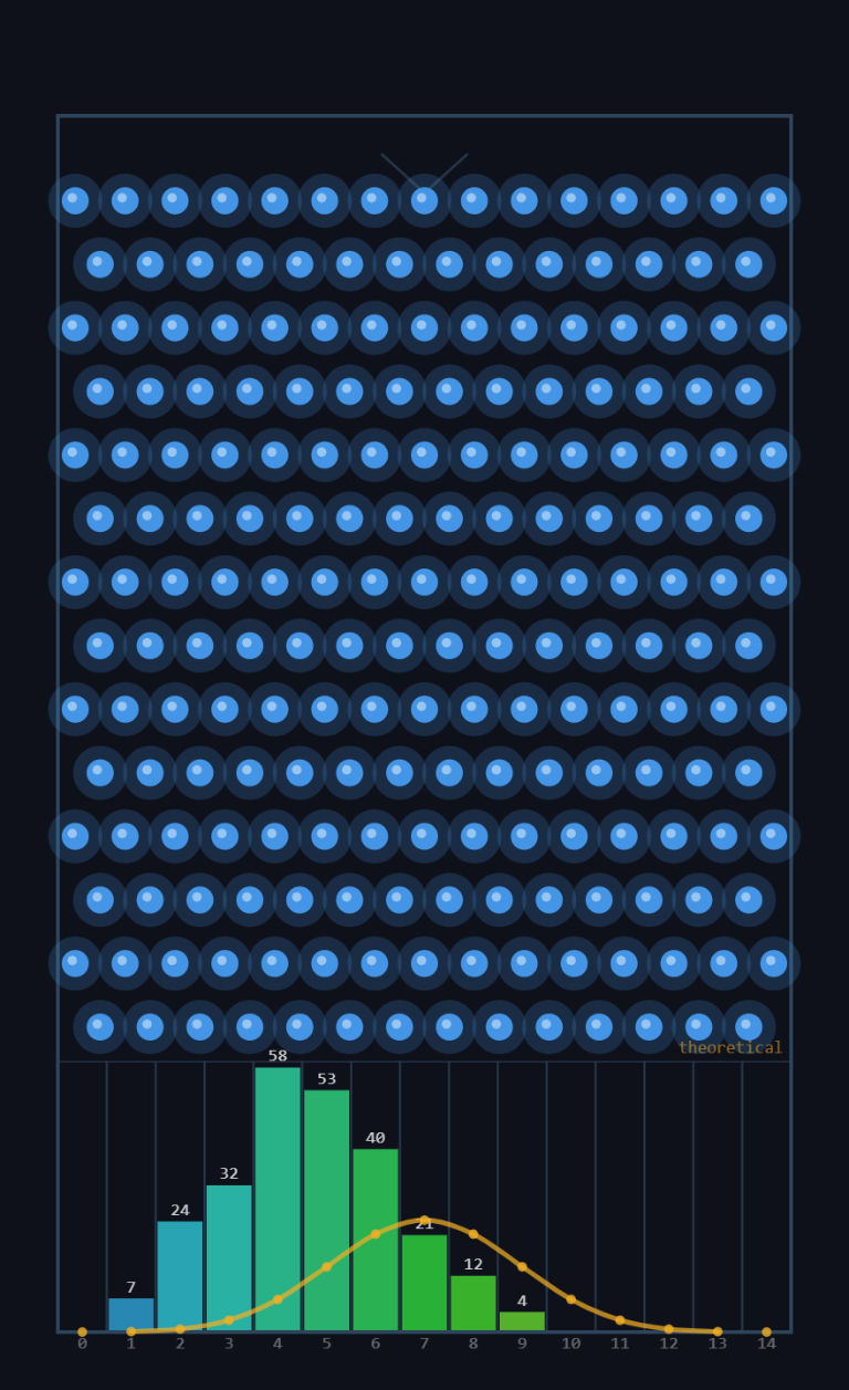
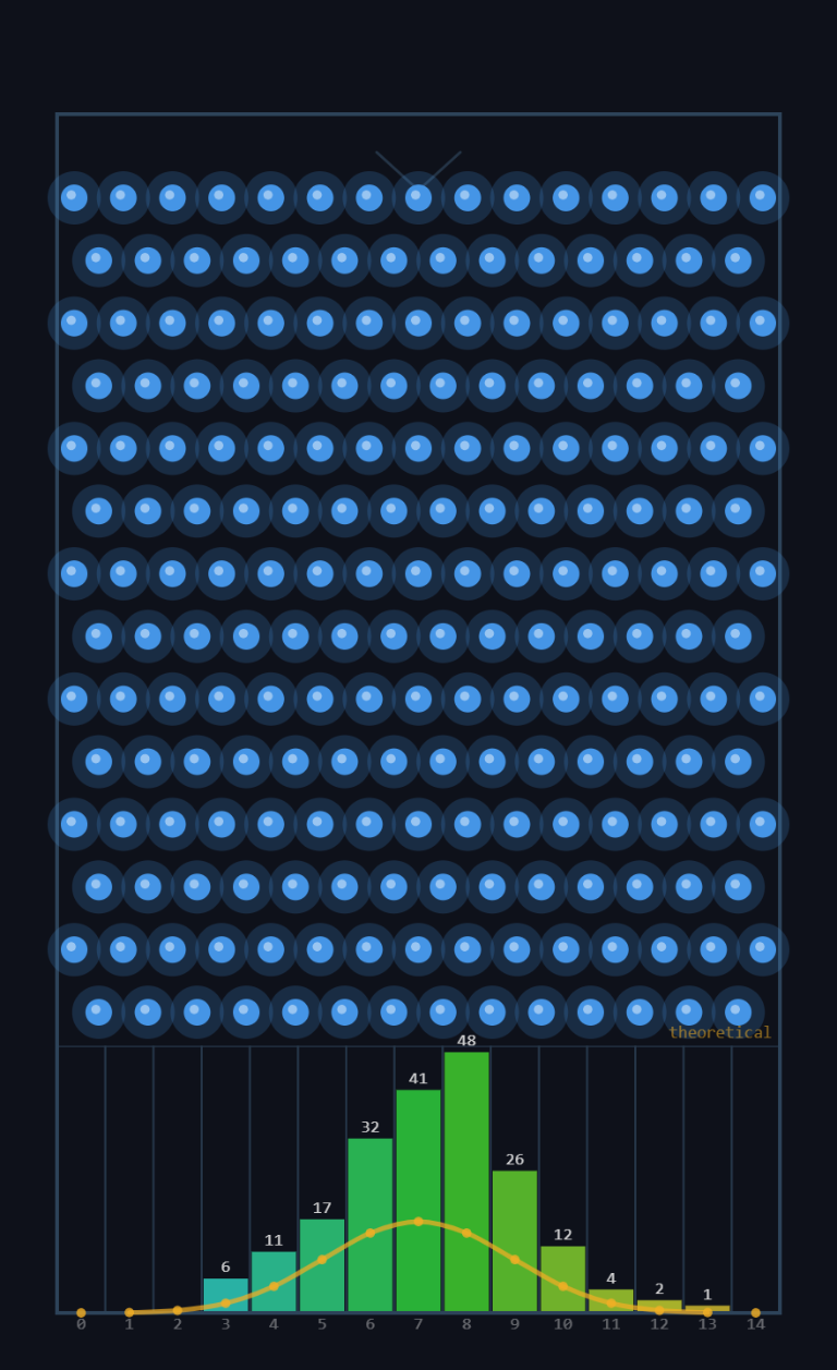
This bug has a crucial teaching dimension. The bias was invisible under most settings:
- 13 rows, same radii — no bias. With 13 rows, peg spacing = 362/13 ≈ 27.8 px and peg surface gap = 27.8 − 14 = 13.8 px. Ball diameter = 12 px < 13.8 px → ball fits cleanly → no double-collisions → no bias.
- 14 rows, ball radius 5 — no bias. Ball diameter = 10 px < peg gap 11.86 px → same reason.
- 14 rows, ball radius 6 — biased. Exactly ONE combination triggered the bug. Every other test looked fine.
This is the most dangerous category of software bug: one that is invisible in most configurations but catastrophic in specific ones. A developer who tested only with the default settings (ball 5, peg 7) would have shipped a simulator that appeared to work perfectly — and would have produced subtly wrong statistics for any user who adjusted radii to larger values.
“We need to be sure to explore multiple settings to ensure the app is valid in multiple states!” — KLP
The standard in professional software is edge-case testing: deliberately test combinations at or near known boundaries (here, the threshold where ball diameter exceeds peg gap). The diagnostic rule that emerged from this session: whenever 2 × ballRadius > rSpacing − 2 × pegRadius, double-collisions become possible and the board can develop systematic bias. Any simulation claiming statistical validity should verify that this inequality does NOT hold for its published settings.
This simulation was first inspired by a few scenes from Stranger Things where Eleven was attempting to influence the results of disks falling through a series of pegs. Research led me to discover its name and some history: the Galton Board. I have two movie clips I’d like to showcase for the idea and link to our app. Please add a movie clip page and cross-link it. Some brief history about the Galton Board’s use in Stranger Things, Galton himself, and why the Galton Board is a prominent idea in probability and statistics.
- movie_clips/galtonBoardInspirationMC.html — new movie clip page following the
babySharkMC.htmltemplate. Navy/gold palette, hero background fromrobotGaltonBoard2.jpg. Three expandable sections: (1) Sir Francis Galton and his bean machine, (2) Stranger Things — Eleven and the peg board experiment, (3) TNT connection and simulator features. Two embedded clips. - movie_clips.html — new grid card with the red bell-curve probability icon, linked to the new page.
- galtonBoardSimApp.html SPARK bar — Movie Clips link added.
- galtonBoardSimAppChatlog.html back-bar — Movie Clips link added.
- bellCurveTutorial.html SPARK bar — Movie Clips link added.
- images/noun_probability_7969006_FF001C_@128.png — red bell-curve icon copied to root images folder for use in the movie grid.